Partial Least Squares (PLS)
Overview
What is Partial Least Squares (PLS)?
Imagine you're running a water treatment plant and want to understand how various operational parameters (like pH levels, flow rates, and chemical dosages) influence the quality of the treated water (e.g., clarity and contaminant levels). Partial Least Squares (PLS) helps by identifying the key relationships between these inputs and outputs, simplifying complex interactions into actionable insights.
PLS is a statistical method used to find relationships between two datasets by creating new features (called components) that summarize the most relevant information from both datasets. These components maximize the correlation between the predictor variables (e.g., operational parameters) and the response variables (e.g., water quality metrics).
How PLS Works for Analyzing Data in Industrial Applications
PLS is especially useful when dealing with datasets where the predictors and responses are numerous and highly correlated. It simplifies the data into components that capture meaningful relationships, making it easier to interpret and predict outcomes.
Example: Imagine monitoring a water treatment plant's operations. PLS can identify which parameters (e.g., flow rate, chemical dosage) most strongly affect water quality metrics like turbidity or contaminant removal, helping operators fine-tune the process for better results.
Example: Consider a situation in which a variable is measured at some times, but is not available at other times. PLS can provide soft-sensing, whereby the values of the missing measurement (the response variable) are reconstructed from other measurements (the predictor variables).
Using the Partial Least Squares Tool
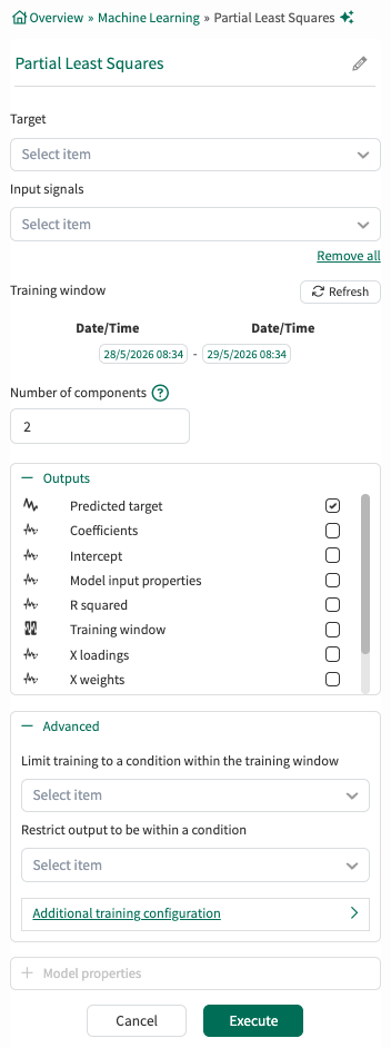
Target: From the dropodown menu, select one signal that will be the response variable of the PLS model.
Input Signals: From the dropdown menu, select at least one signal to serve as the predictor variable(s) for the model.
Training window: Select the fixed window of data on which the model will be trained. If no limiting condition is selected in the Advanced section, the training window defaults to the display range of the worksheet. The Refresh button can be used to update the Training window.
Number of components: The number of components cannot exceed the number of input signals. Too many components leads to overfitting which is when a model learns too much from the specific details and noise in the training data, leading it to be overly sensitive. This results in a model that performs well on the training set but poorly on test or validation data. In this example, the user has chosen to use two PCs.
Outputs:
Lists all outputs available for the current tool configuration. Choose which outputs the tool should generate and add to Trend. Default outputs are preselected, and additional supported outputs can be selected as needed. For detailed descriptions of each output, see the output documentation.
Advanced:
Limit to condition within training window: You can choose to limit the data supplied for training to data from within the training window and within a condition. For example, you could choose a condition that identifies when an operation is running. All data outside of the condition (when the unit is not running) will be ignored for the model training.
Restrict output to be within a condition: You can limit the data displayed to only show results within a relevant condition. If you limit the training to periods of time when the unit is running, you might want to restrict the output to the same running condition.
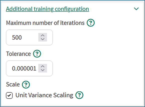
Additional training configuration:
Maximum number of iterations: Defaults to 500. PLS is an iterative algorithm where each component is the result of a number of iterations. Commonly a stable solution is found with fewer than 500 iterations. Increasing the maximum number of iterations may result in increased training time but can yield better results.
Tolerance: Defaults to 10-6. The tolerance is used as a convergence criterion: the algorithm stops iterating when the improvements to the new result are below a value proportional to the tolerance.
Scale: Defaults to true. By default all variables are centered and scaled to unit variance by subtracting the signal average from each data point and dividing by the signal standard deviation. This is appropriate pre-treatment for process data since it removes units of measure and will give an equal chance to all input signals to influence the model regardless of the actual numerical values.
There are cases when unchecking this box is appropriate such as if all input signals have the same units of measure and are already related to a shared reference other than the signal average.
Example of a PLS analysis
The image below shows an example in which the PLS model was trained to output Temperature as the response variable from Compressor Power, Relative Humidity, and Wet Bulb as the predictor variables. The dataset used for training comprises the values of these measurements within the capsules of the Stage 1 condition that are highlighted with the beige color. The PLS tool builds a model that can determine the Temperature from the values of the three other measurements.
The trained PLS model is then applied to other periods of operation. During these periods, the orange signal called ‘PLS Demo - Temperature model’ in the lowest lane is being calculated from Compressor Power, Relative Humidity, and Wet Bulb using the trained PLS model. The actual temperature is shown in a dark blue color for comparison.
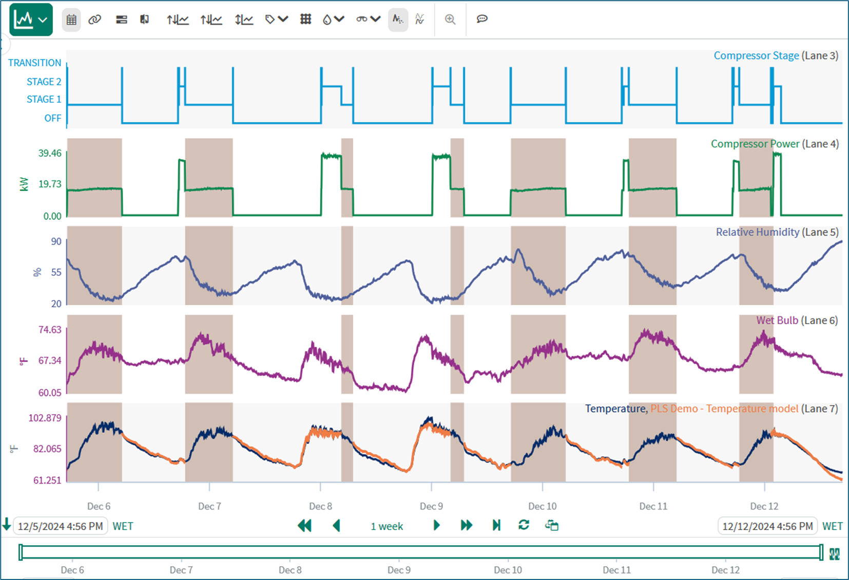
PLS model for Temperature. Beige capsules - training data; Orange signal - model output; Dark blue signal - actual temperature.
Model properties
The PLS tool provides detailed information that can be viewed by expanding the Model Properties section:
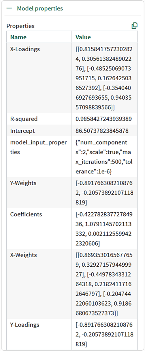
R-squared
The R2 value quantifies how much of the behavior of the output signal the model reproduced during training. The maximum value is 1.
Model Input Properties
The model_input_properties variable confirms the training configuration.
Coefficients and Intercept
The PLS model is linear with the form:
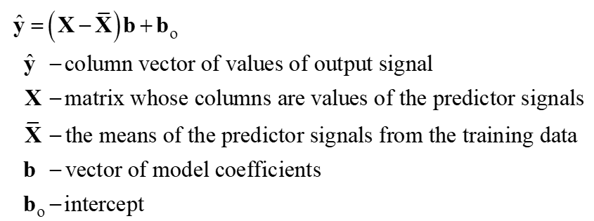
The Coefficients and Intercept are calculated during training. The PLS calculations take into account that the columns of the X matrix may be correlated with each other and with the output signal. Intermediate steps in the calculation are X-Loadings, X-Weights, Y-Loadings, and Y-Weights. The attributes of these quantities are explained here.
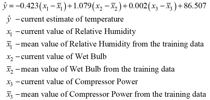
Numerical example
To three decimal places, the Properties table shows the values of the Coefficients are -0.423, 1.079 and 0.002, and the Intercept is 86.507. Applied to the earlier worked example, the model is:
Use Cases for Partial Least Squares in Key Industries
Manufacturing and Production Optimization
PLS helps manufacturers understand and improve the relationships between process parameters and product quality:
Process Control: Identifying which process variables (e.g., temperature, pressure) most impact product consistency.
Yield Optimization: Predicting and maximizing production output by adjusting key variables.
Pharmaceutical Development and Quality Control
In pharmaceutical environments, PLS enables the development and control of robust manufacturing processes:
Formulation Development: Linking ingredient properties with drug efficacy to optimize formulations.
Quality Assurance: Detecting process variations that may lead to out-of-specification products.
Chemical and Petrochemical Processes
PLS supports complex systems with many interacting variables by isolating the critical ones:
Process Optimization: Pinpointing which variables have the greatest impact on efficiency or yield in refining or chemical synthesis.
Emissions Reduction: Understanding the relationships between input variables and pollutant levels to minimize environmental impact.
Semiconductor Manufacturing
PLS helps in improving process stability and product reliability:
Defect Analysis: Linking sensor data with defect rates to identify root causes of failures.
Recipe Optimization: Relating process recipes to chip performance metrics for higher yields.
Energy and Utilities
PLS supports predictive analysis and optimization in energy generation and distribution:
Power Plant Efficiency: Identifying how changes in fuel composition or operating conditions impact efficiency and emissions.
Water Treatment Optimization: Relating operational parameters to water quality metrics, enabling fine-tuned processes for better results.
Benefits of Partial Least Squares
Handles Multicollinearity: PLS is robust when predictors are highly correlated, which is common in industrial data.
Dimension Reduction: It reduces the complexity of large datasets by creating fewer, meaningful components.
Predictive Power: PLS provides interpretable models that predict outcomes based on key relationships in the data.
A Few Limitations of PLS
While PLS is a powerful tool, it has some limitations:
Interpretability of Components: The new features (components) are combinations of the original variables, which may require extra effort to interpret.
Sensitivity to Noise: If the data contains noise, PLS components may capture irrelevant patterns, affecting predictions.
Requires Tuning: The number of components to include must be carefully selected to avoid underfitting or overfitting the model.
Notes on training the model
The data from the input signals that goes into training is auto gridded. This means that the samples from all the signals are aligned - same sampling rate across the training window. Each input signal will be resampled to have the same number of samples in the training window.
The signals may get down-sampled if the total number of samples in the training window is greater than 2.5 million.