Signal Forecast
The Signal Forecast tool enables users to forecast signals beyond their known data using a variety of techniques to create signals beyond the source data for predictions and boundary management.
Using the Signal Forecast tool
The Signal Forecast tool can be opened from the tools panel under the Model & Predict section. The basic UI contains a signal selection input and a selection for the type of algorithm to use for the forecast with Linear as the default.
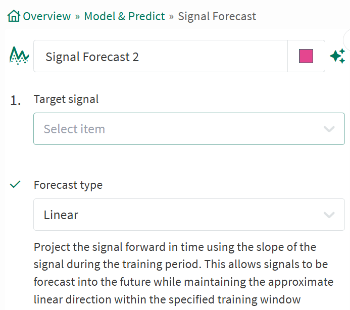
Basic UI Input for the Forecast
Target signal: From the dropdown menu, select the signal you want to forecast.
Forecast type: From the dropdown menu, select the type of forecast algorithms to use. A brief description of the forecast type selected will show below the input.
Forecast Linear
Setting the forecast type to Linear will project the signal forward in time using the slope of the signal during the training period. This allows signals to be forecast into the future while maintaining the approximate linear direction within the specified training window. A linear forecast can also be performed directly from formula by calling .forecastLinear() on the signal to be forecasted.
This uses an Ordinary Least Squares regression to calculate the time-weighted slope based on the raw (ungridded) samples of the input signal. The forecasted values are considered uncertain and will be updated as new certain samples arrive in the signal. A maximum of 10,000 samples are allowed in the training window. Invalid training samples are ignored.
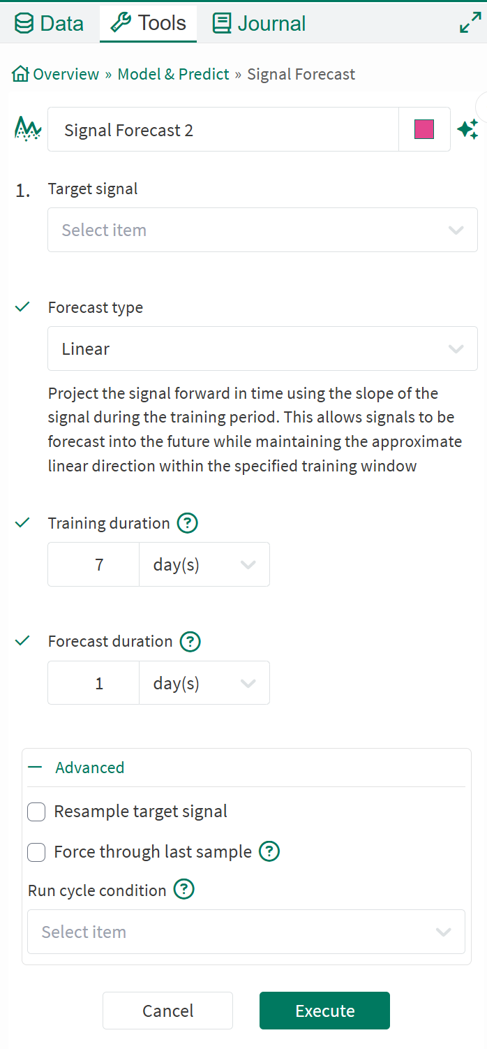
Forecast Linear
Training Duration: Select the amount of time before the last certain sample to train the regression model with. The default value is 7 days but can be modified. The training window is inclusive of both ends of the duration.
Forecast Duration: Select the length of time the forecasted signal will cover. This is the amount of time past the last certain sample to linearly extrapolate the data.
Advanced Options:
Resample target signal: When checked, it allows you to select a resampling rate for the target signal. This will convert the signal to the specified sampling rate before applying the forecast algorithm, while preserving as much of the original signal's data as possible.
Force through last sample: This indicates whether the prediction model should pass through last sample and begin the forecast at the same location. True will calculate a prediction that is influenced more heavily by the last sample and will result in a continuous forecast joined with the certain data. False will result in an evenly-weighted prediction with a gap between the certain data and the forecast.
Run cycle condition (Cannot be used together with force through last sample): Optionally select a condition for which the training window will be truncated to correspond to latest capsule's start in that condition. This can be visualized as:
CODEsignal: ~~~~~~~~~~~~~~~~~~~~~~ traininDuration: ├──────────────┤ runCycle: ├───┤ ├────── actualTraining: ~~~~~~~If no capsules start in the that window, the entire
trainingDurationwill be used.
Forecast Constant
Setting the forecast type to Constant will project the last value of a signal forward in time. This allows signals to forecast in the future without changing the maximum interpolation of the signal. The forecasted values are considered uncertain, and will be updated as new samples arrive in the signal.
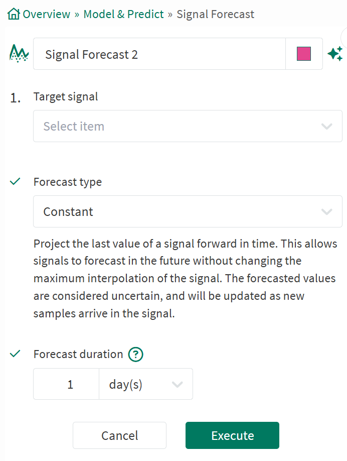
Forecast Constant
Forecast Duration: Select the length of time the forecasted signal will cover. The amount of time past the last certain sample to hold the value. Default value is a day
Forecast ARIMA
Setting the forecast type to ARIMA will project the signal forward in time using forecasting based on ARIMA models. When seasonality shows in the time series, the seasonal-differencing could be applied to eliminate the seasonal component. This type of forecasting should be applied in cases where the data shows evidence of non-stationarity. The parameters of the model are estimated using the Hannan-Rissanen algorithm. The forecasted values are considered uncertain and will be updated as new certain samples arrive in the signal. The predictor assumes uniform sampling rate. A maximum of 100,000 samples are allowed in the training window. More detailed usage guidelines are available in the Knowledge Base.
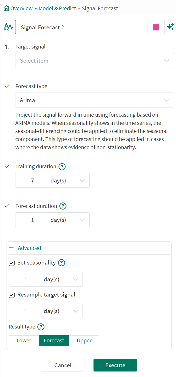
Forecast ARIMA
Training Duration: Select the amount of time before the last certain sample to train the regression model with. The default value is 7 days but can be modified. The training window is inclusive of both ends of the duration.
Forecast Duration: Select the length of time the forecasted signal will cover. This is the amount of time past the last certain sample to extrapolate the data.
Advanced Options:
Set seasonality: When checked, it allows you to select a period of the repeating pattern found in the data.
Resample target signal: When checked, it allows you to select a resampling rate for the target signal. This will convert the signal to the specified sampling rate before applying the forecast algorithm, while preserving as much of the original signal's data as possible.
Result type: Select the type of samples returned by the algorithm. Possible values are 'upper', ' lower' and 'forecast' (default value). The upper and lower bounds correspond to the 95% confidence interval.
Forecast Splice
Setting the forecast type to Splice enables the splicing or the chaining of two signals together at the time of the last certain value of the first signal. This enables known historical performance (first signal) to be combined with forecasts and models of future performance (second signal) into a single continuous signal.
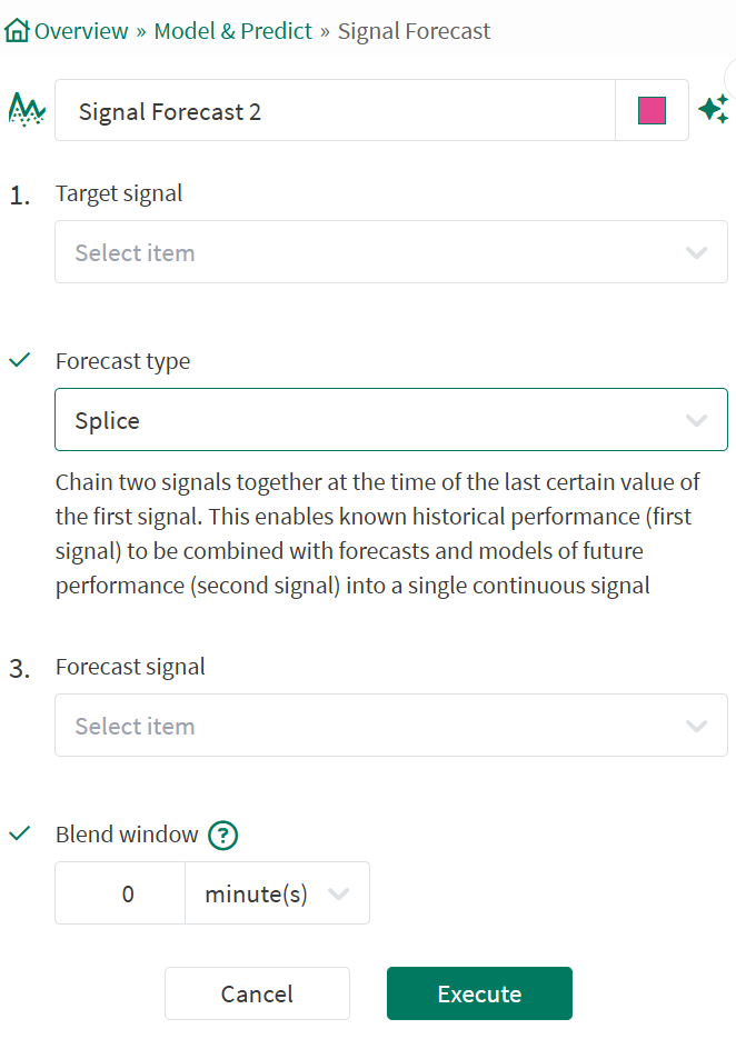
Forecast Splice
Target Signal: Select the historical signal to be spliced with the forecast signal.
Forecast Signal: Select the forecast signal to chain with the target (historical) signal.
Blend Window: Select the time duration over which to scale the forecast signal when there is a discontinuity between the two signals. Defaults to 0 seconds.