Self Organizing Maps (SOM)
What is a Self-Organizing Map (SOM)?
Imagine you're organizing a messy room. You start by grouping similar items together: clothes in the closet, books on the shelf, and toys in the toy box. A Self-Organizing Map (SOM) works similarly, but with data points instead of physical objects.
In simpler terms, a SOM is a type of artificial neural network that organizes data into a 2D grid. Each node on the grid represents a specific pattern or cluster of data points. Over time, the SOM learns to group similar data points together, creating a visual representation of the underlying patterns.
How SOMs Work for Detecting Anomalies in Time Series Data
In time series data, detecting anomalies is all about spotting when something doesn’t follow the usual pattern. SOMs do this by learning what “normal” looks like based on previous data. Once the SOM has a good idea of these regular patterns, it can monitor new data and alert when something unusual happens.
Example: Imagine a manufacturing machine that runs continuously. A SOM trained on the machine's normal behavior can pick up on changes in the machine's data that might suggest a problem, such as vibrations or temperature spikes. If the SOM detects data that looks very different from what it has learned, it can flag this as an anomaly, signaling the need to check the machine before it breaks down.
Using the Self Organizing Map Tool
Find the Self Organizing Map Tool under the Machine Learning section of the Tools Pane, or use the “Filter Tools” text box .
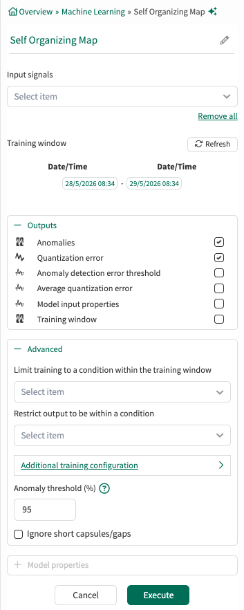
Input Signals: From the dropdown menu, select at least one signal to serve as independent variable(s) for the model.
Training window: Select the fixed window of data on which the model will be trained. This defaults to the display range but can be modified.
Outputs:
Lists all outputs available for the current tool configuration. Choose which outputs the tool should generate and add to Trend. Default outputs are preselected, and additional supported outputs can be selected as needed. For detailed descriptions of each output, see the output documentation.
Advanced Options:
Limit to condition within training window: You can choose to limit the data supplied for training to data from within the training window and within a condition. For example, choose a condition that identifies when an operation is running and all data outside of the condition (when the unit is not running) will be ignored for the model training.
Restrict output to be within a condition: You can limit the data displayed to only show results within a relevant condition. If you limit the model to periods of time when the unit is running, you would likely want to restrict the output to the same running condition. You can use different condition here than the training window if appropriate.
Anomaly threshold: When a condition is the selected output, apply a threshold between 0 and 100. Higher values will result in fewer anomalies detected, but you may need to iterate to ensure you are finding the appropriate anomalies. The threshold indicates how much of the training data one expects to be an anomaly.
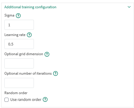
Additional training configuration
This section lets users configure advanced model parameters when reviewing results and iterating to obtain a fine tuned model. These parameters are related to how training is done and are specific to the SOM algorithm.
Sigma: This defaults to 1. During training this value is used to determine how far is the area of effect of the winner node. The larger the value, the more nodes are impacted,
Learning rate: This defaults to 0.5. During training, this value is used to determine how much the winning node moves toward the sample. Lower values can lead to nodes finding a better cluster center position, but training may need more iterations to ensure the cluster center is found.
Optional grid dimension: This defaults to a value computed based of the number of input samples. The value represents the size of the grid. The number of nodes in the SOM is this number squared. The number of nodes should reflect how many clusters are expected in the training data.
Optional number of iterations: This defaults to a value computed based on the grid dimension. The value represents how many iterations of adjusting the node positions are executed. Increasing the number may lead to better precision but will increase the training duration.
Using random order: This defaults to false. The flag represents whether to shuffle the data when doing epochs of training. Making this true will lead to a more stochastic training.
Use Cases for Self-Organizing Maps in Key Industries
Manufacturing and Production Monitoring
SOMs help detect early signs of issues by identifying deviations from normal operating patterns, helping to reduce downtime and improve quality:Equipment Maintenance: Monitoring vibration, temperature, or pressure data to spot early signs of wear or failure in machinery.
Product Quality Control: Identifying irregular patterns in production data that could indicate quality issues, enabling corrective action before the product is shipped.
Pharmaceutical Manufacturing and Quality Assurance
In highly regulated environments like pharmaceuticals, consistency is key. SOMs can detect process variations that may impact product quality:Batch Consistency Monitoring: Ensuring that each batch follows the same profile by flagging deviations in temperature, mixing times, or ingredient ratios.
Environment Control: Detecting anomalies in humidity, temperature, or cleanroom conditions that could impact sensitive production processes.
Chemical and Petrochemical Processes
Chemical engineering processes involve complex systems that require careful monitoring of variables like pressure, flow rates, and chemical composition:Process Optimization: Recognizing normal operating patterns for reactors or distillation columns and flagging deviations to avoid costly production losses.
Safety Monitoring: Identifying unusual pressure or temperature changes that could signal leaks or unsafe conditions, allowing for quick intervention.
Semiconductor Manufacturing
Semiconductor production is a precision-driven process where even small anomalies can impact yield and performance:Defect Detection: Flagging unusual readings from sensors monitoring cleanroom environments, such as particle count or chemical purity, which may indicate contamination.
Process Stability: Monitoring the consistency of etching or deposition processes, where small changes could lead to defective chips.
Energy and Utilities
Energy providers rely on continuous monitoring of systems like turbines, pipelines, and grids. SOMs can help detect early warning signs in these critical systems:Pipeline Monitoring: Detecting changes in flow or pressure in pipelines that could indicate leaks or blockages.
Power Grid Health: Identifying unusual patterns in load distribution or voltage levels, helping prevent outages or equipment stress.
Utilities and Renewable Energy
For utilities, maintaining stable operations and spotting issues early helps keep systems efficient and reliable:Wind Turbine Monitoring: Identifying changes in vibration or load patterns to predict maintenance needs and prevent unexpected downtime.
Water Treatment Plants: Monitoring water quality metrics to detect any deviations that could impact the purification process or output quality.
Benefits of Self-Organizing Maps
Clear Pattern Visualization: SOMs simplify complex data into visual patterns, making it easier to understand trends and spot anomalies.
Flexible, Label-Free Operation: SOMs don’t require labeled data, which makes them suitable for environments where patterns are complex or not predefined.
Scalability: SOMs handle large datasets efficiently, so they’re useful for industries with high volumes of data from sensors and monitoring equipment.
A Few Limitations of SOMs
While SOMs are powerful, they’re not ideal for every situation:
Training Time: SOMs can take time to learn from data, especially if the dataset is large.
Trial and Error in Map Design: Finding the ideal map size may require testing to achieve the best results.
Less Suitable for Labeled Data: SOMs are best for finding patterns, rather than making specific, labeled predictions.
Notes on training the model
The data from the input signals that goes into training is auto gridded. This means that the samples from all the signals are aligned - same sampling rate across the training window. Each input signal will be resampled to have the same number of samples in the training window.
The signals may get down-sampled if the total number of samples in the training window is greater than 2.5 million.