Principal Component Analysis (PCA)
Overview
What is Principal Component Analysis (PCA)?
Principal Component Analysis (PCA) identifies typical patterns in signals and detects deviations from normal behavior. It is used to monitor for anomalous conditions based on historical data from normal operation. The Principal Component Analysis (PCA) is a dimensionality reduction and machine learning method used to simplify a large data set into a smaller set that retains most of its original and valuable information.
PCA transforms a set of correlated variables into a smaller set of uncorrelated variables called principal components. The first principal component captures the most variance in the data, the second one captures the next most, and so on. Physically, a principal component represents a typical plant profile, for instance that certain variables tend to deviate from their average in one direction while others deviate in the opposite direction.
How Principal Component Analysis works in Time Series Data
Imagine you're monitoring a distillation column in a chemical plant. You’re collecting data from several sensors: temperature at different stages, pressure, flow rates, composition of the top and bottom products, and maybe even ambient conditions like room temperature or humidity.
That’s a lot of variables, and many of them are related—for example, if the reboiler temperature increases, the bottom product composition might change too.
Now you want to figure out if the process is running normally or if something unusual is happening. Looking at all these variables individually is hard and time-consuming.
This is where PCA comes in.
PCA takes all those sensor readings and finds patterns in how they change together under normal conditions. It then creates a few new “super variables” (principal components) that summarize most of the important information in the process.
The first principal component might capture overall heat balance—combining temperatures and energy input.
The second principal component might represent product purity and its relationship to flow rates or reflux ratio.
A third might capture minor variations in ambient conditions.
Once PCA is trained on normal operation data, you can plot new incoming data in terms of these components. If something shifts in a way that doesn't fit the usual pattern—like a valve sticking or a sensor drifting—PCA will show that the system is behaving unusually, even if none of the individual sensors look far out of range.
In Seeq we do this by computing a log-likelihood monitoring signal based on the PCA model outputs, which measures whether a new plant profile fits within the normal patterns learned during training, or if the profile is likely to be anomalous. A high log-likelhood value indicates that the current profile deviates significantly from normal operation and may be an anomaly.
To aid interpretation, the model presents the loadings matrix, which contains the principal components. The principal components are building blocks: each plant profile can be approximately reconstructed using a weighted linear combination of these components. This makes it easier to understand which signals contribute most to variations in the process, and to identify which changes might be driving anomalous behavior.
Using the Principal Component Analysis tool
The PCA tool can be opened from the tools panel under the Machine learning section, or by searching on the “Filter Tools” text box.
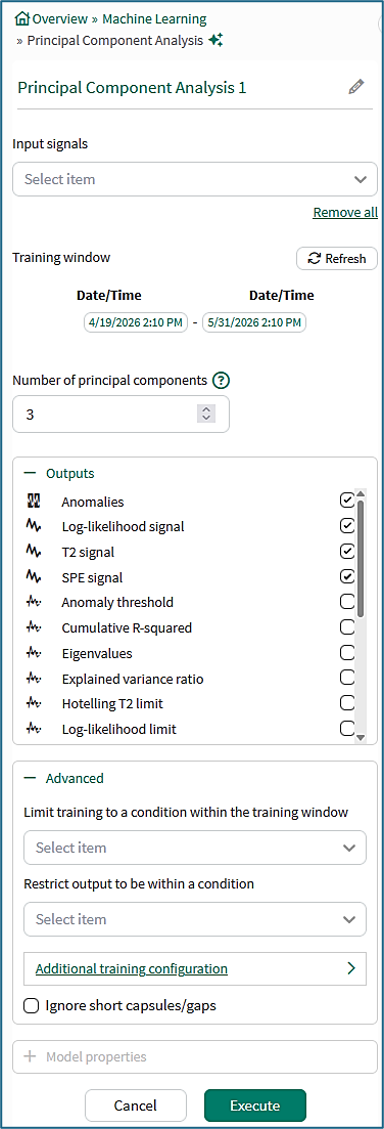
Input signals: From the dropdown menu, select at least one signal to serve as variable(s) for the model.
Training window: Select the fixed window of data on which the model will be trained. If no training condition is selected in the Advanced section, the training window defaults to the display range of the worksheet.
Number of principal components: Defaults to 3 and cannot exceed the number of input signals. Too many components leads to overfitting which is when a model learns too much from the specific details and noise in the training data, leading it to be overly sensitive. This results in a model that performs well on the training set but poorly on test or validation data. The number of principal components determines the dimensionality reduction which in turn impacts how much of the variance of the original data you retain.
Outputs:
Lists all outputs available for the current tool configuration. Choose which outputs the tool should generate and add to Trend. Default outputs are preselected, and additional supported outputs can be selected as needed. For detailed descriptions of each output, see the output documentation.
Advanced:
Limit to condition within training window: You can choose to limit the data supplied for training to data from within the training window and within a condition. For example, choose a condition that identifies when an operation is running and all data outside of the condition (when the unit is not running) will be ignored for the model training. Here, the user is training on a condition called Training.
Restrict output to be within a condition: You can limit the data displayed to only show results within a relevant condition. If you limit the model to periods of time when the unit is running, you would likely want to restrict the output to the same running condition. You can use a different condition here than the training window if appropriate.
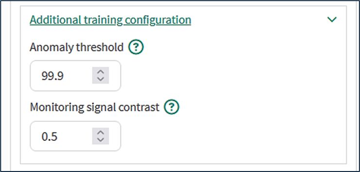
Additional training configuration:
Anomaly threshold: Defaults to 99%. Higher values will result in fewer anomalies detected, but you may need to iterate to ensure you are finding the appropriate anomalies. The threshold indicates how much of the training data one expects to be anomalous. For instance, a model trained with the default anomaly threshold of 99% will show an average of one anomaly for every 100 samples in the training data. In this example, the user has selected 99.9%, so the PCA model will show one anomaly for every 1000 samples in the training set.
Monitoring signal contrast: Applies to the Loglike monitoring signal only and defaults to 0.5. Higher values of monitoring contrast give more abrupt transitions in the log-likelihood monitoring signal, lower values show more gradation in behavior. The monitoring signal contrast can take values between 0 and 5.
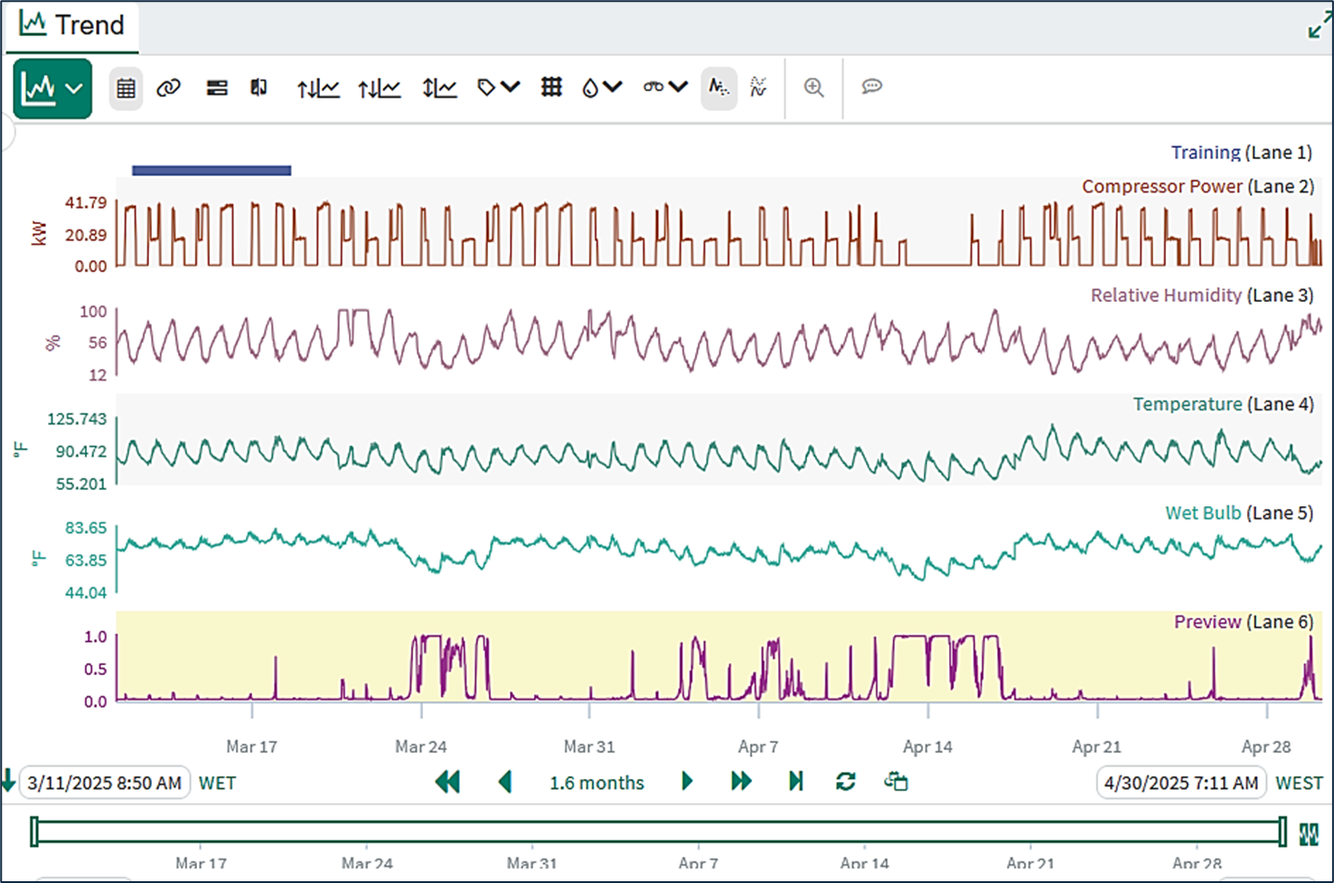
Preview view
Example of a full analysis
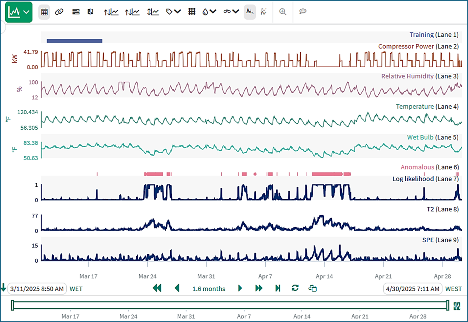
The image below shows an example in which the PCA model was trained with two principal components on the signals under the capsule in the Training condition. The outputs shown are the Anomalous condition, Seeq’s Loglike monitoring signal that detects all anomalies, and the classic T2 and SPE monitoring signals.
The Log likelihood (Loglike) monitoring signal is high in March 24th and 25th, around April 14th and on one or two other occasions. Visual inspections show that, for the 24-25th March episode, the anomaly arises because values for the Wet Bulb signal are much lower than any Wet Bulb values included in the Training set on the left hand side of the trend view. Values for Relative Humidity are also on the low side. The anomalies in the April 14th episode include lower values for the Wet Bulb and also a flat line in the compressor power of much longer duration than any seen in the training set.
The values of the T2 monitoring signal are raised during these episodes. Higher T2 values mean that the correlations and relationships between variables detected during training of the PCA model are still intact, but the numerical values involved are outside of those encountered during the training period. Specifically, the T2 is raised because the relationship between Wet Bulb and Relative Humidity is still intact but the values are extremely low.
The SPE monitoring signal is raised if correlations and relationships detected during training of the PCA model are no longer present. In the example PCA analysis, SPE becomes periodically high in the anomalous episode around April 14th.
During the training period, the off-on behavior of the Compressor Power signal aligned with the peaks and valleys of the oscillating process signals, for instance during the Training period, Temperature and Wet Bulb have a valley and Relative Humidity has a peak when Compressor Power is zero. This relationship periodically breaks down in the episode around April 14th. At that time, there are instances when Temperature and Wet Bulb have a peak and Relative Humidity has a valley when Compressor Power is zero. This is an unusual combination is not present in the trained PCA model, and hence the SPE monitoring signal is raised.
PCA Hint: If the Log likelihood monitoring signal is persistently above its 0.5 limit and the SPE signal is persistently above its SPE Limit, this may indicate that there are not enough Principal Components in the trained model.
PCA analysis with anomaly detection
Model Properties
The PCA tool provides detailed information that can be viewed by expanding the Model Properties section:
Properties tab
Model properties
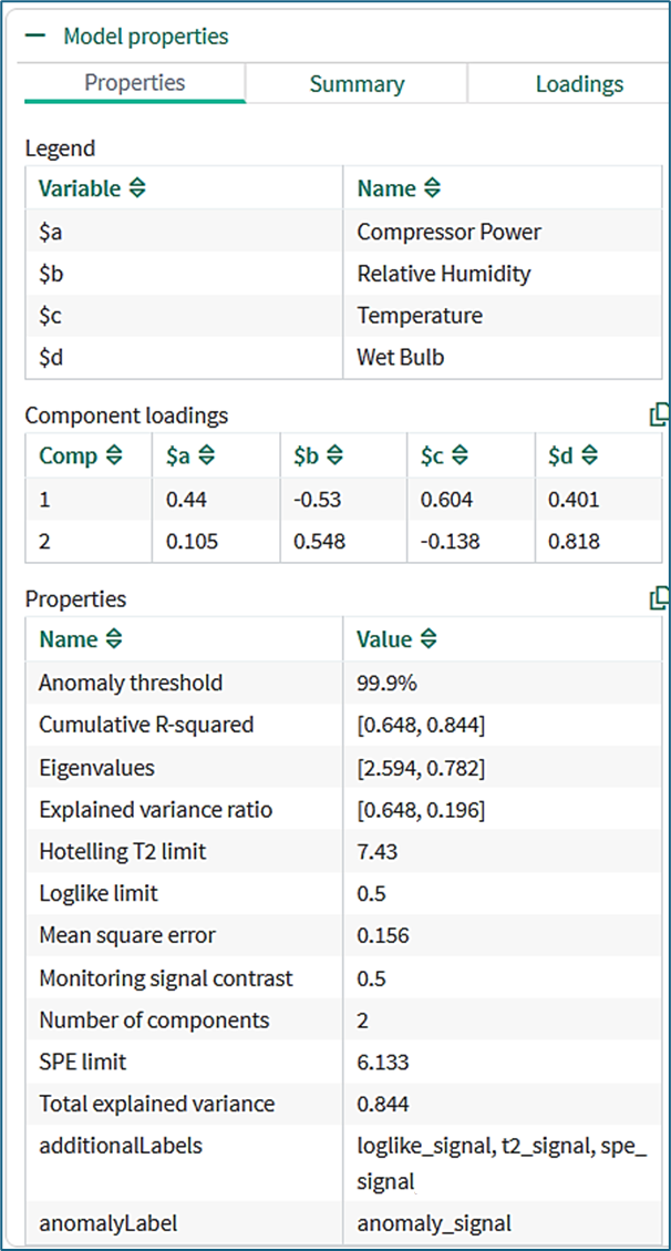
Legend: Maps input signal names to column headings in the Component loadings table.
Component loadings: The PCA loadings for each principal component of the calibrated model.
Properties: Displays model metadata in alphabetical order, including:
Cumulative R-squared: Indicates how explanatory power of the PCA model builds as principal components are added.
Eigenvalues: The variance explained by each principal component. Larger eigenvalues correspond to the most significant principal components.
Explained Variance Ratio: Indicates the proportion of the total variance in a dataset that is explained by each principal component.
Hotelling T2 limit: A statistical threshold for the T2 signal used to assess whether an observation is considered anomalous, or is within the expected range of the model.
Loglike limit: An anomaly is identified if the log likelihood signal exceeds 0.5 (this is independent of the Monitoring signal contrast. The similarity of their numerical values is just a coincidence). The log likelihood signal for a model trained with an anomaly threshold of 99.9% will exceed 0.5 for one in every 1000 samples of the training data.
Mean Square Error: Measures the average squared difference between the original data points and their projections onto the principal components.
SPE (Squared Prediction Error) limit: A statistical threshold for the SPE signal used to assess whether an observation is considered anomalous, or is within the expected range of the model.
Total Explained Variance: The sum of explained variances for all individual principal component. You can copy both component loadings and model properties to the clipboard for further analysis.
Summary tab
The Summary tab contains a combined chart of the Explained variance ratio and the Cumulative R-squared values.
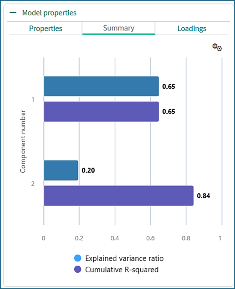
Summary chart
The Explained Variance Ratio chart (blue-green bars) refers to a visualization that displays the Explained Variance Ratio (EVR) for each principal component (PC). This chart helps determine how much variance in the training data set is captured by each PC, aiding the selection of the optimal number of components for dimensionality reduction
The Cumulative R-squared (R²) chart (blue bars) shows the proportion of variance in the data that is explained by the principal components (PCs). A higher cumulative R² value indicates that the PCs capture a greater amount of the variability of the training dataset.
The EVR and cumulative R² are related. The cumulative R² value for any component is the sum of the EVR values up to and including that component. (Verification of this from the numerical values in the chart may be affected by the limited number of decimal places.)
Loadings tab
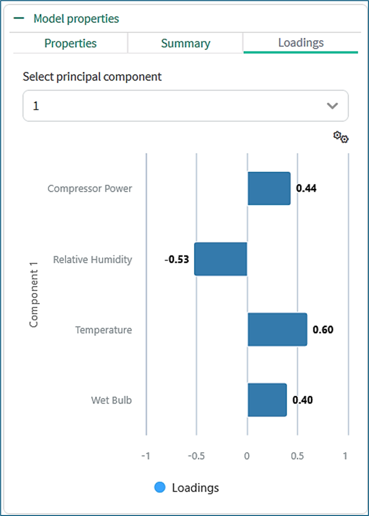
Loadings Chart for PC 1
The loadings tab shows a loadings chart that visualizes the relationship between the original variables (in this case, signals) and the resulting principal components (PCs). It shows how strongly each signal contributes to each PC, essentially demonstrating which variables are most influential in defining each component.
The plant profiles during normal operation can be reconstructed from a weighted sum of the loadings. The image shows that Principal Component 1 captures a common plant profile where Temperature, Wet Bulb, and Compressor Power deviate from their average values in one direction, while Relative Humidity deviates from its average value in the opposite direction.
The select principal component dropdown allows for the visualization of these signals for each component, i.e., Depending on the selected principal component, the chart will be updated with the corresponding values for each signal.
Chart settings
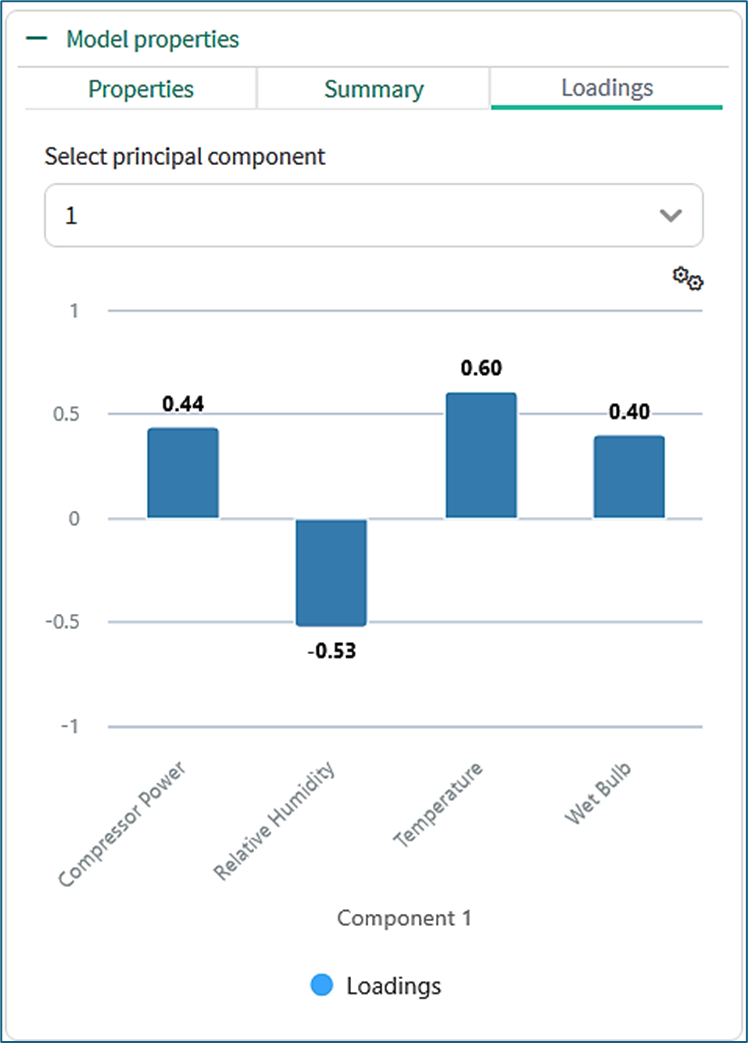
Loadings for PC1 as Column Chart
The Summary and Loadings both have a settings option (the gears icon) to configure the chart for a preferred visualization which includes sorting the values by ascending or descending order, or switching between Bar, Column or a Line chart.
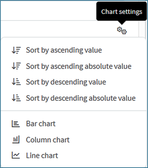
Chart settings menu
Use Cases for Principal Component Analysis in Key Industries
Manufacturing and Production Monitoring
Principal Component Analysis in industrial monitoring finds use in fault detection, outlier detection, and process understanding. It helps to identify anomalies in data, reduce the complexity of datasets, and understand relationships between variables.Fault detection: When the process deviates from normal (e.g., due to a fault), the PCA model will detect deviations, indicating a potential issue. A monitoring signal shows how well the principal components from the trained model can explain the values of the new samples. For example, the PCA monitoring signal becomes large if a thermocouple fails or is dislodged because the deviations from the trained PCA model no longer look like random noise.
Process Understanding: PCA helps understand the relationships between different process measurements and identify which of them contributes most to the observed variability.
Pharmaceutical Development and Quality Control
Principal Component Analysis is a valuable tool in pharmaceutical development and quality control for ultimately aiding in optimizing processes and ensuring product quality.Formulation Development: It can reveal relationships between different variables in a process, helping to understand which factors have the most significant impact on product quality.
Quality Assurance: The early detection of failed batches, typically due to contamination or a failed feed pump.
Chemical and Petrochemical Processes:
Detecting Impurities and Contaminants: PCA can help identify deviations from expected patterns that might indicate the presence of unwanted substances.
Catalytic Process Monitoring: PCA can be used to monitor the performance of catalytic processes, such as in catalytic reformers, and identify potential issues or areas for improvement.
Semiconductor Manufacturing:
Predictive Maintenance: PCA can be used to predict equipment failures by monitoring performance and performance and identifying early signs of degradation.
Energy and Utilities:
PCA offers several use cases in the energy and utilities sector, primarily focusing on data simplification, forecasting, and grid optimization.Improved Forecasting: By identifying the most influential variables, PCA can be used to build more accurate and robust models for energy consumption, demand, and renewable energy generation.
Grid Performance Analysis and Monitoring: PCA helps in analyzing the performance of the electrical grid by identifying key factors influencing load patterns and identifying potential issues or anomalies.
A broader discussion of which ML tool to use for a given purpose can be found in Machine Learning Tools – FAQ.
Benefits of Principal Component Analysis
Dimensionality Reduction: Transforms data into a lower-dimensional space while preserving most of the original variance, making it easier to work with and analyze high-dimensional datasets.
Noise Reduction: By focusing on the most important components, PCA can remove noise and irrelevant information from the data.
Data Visualization: Allows for the visualization of complex datasets in a lower-dimensional space, making it easier to identify patterns and relationships.
Faster Computation: Reduced dimensionality can lead to faster computation times for machine learning algorithms.