
The Operationalize Statistics Summary tool converts an existing Statistics Summary into operational Statistical Process Control (SPC) charts and periodic statistics in the Trend view of Seeq Workbench. It uses the charts configured in the selected Statistics Summary to create outputs for the data in the display range, allowing users to compare current process behavior with an established baseline.
Once operationalized, the baseline statistical analysis becomes a reusable Seeq Template. The tool applies the control chart parameters and statistical tests of the baseline to the data in the current display range and recalculates the outputs whenever that display range changes.
The tool makes it easy to monitor process stability and detect shifts from established norms over time.
Key capabilities:
-
Generation of I-(Individuals) and MR-(Moving Range) control charts
-
Generation of Xbar-(Average) and R-(Range) or S- (Standard deviation) control charts
-
Application of Western Electric (WE1 to WE4) run rules for automated variation detection
-
Periodic calculations of statistics (Cpk, Ppk, and p-values for tests of normality, equal means and equal variances)
-
Customization of timestamp placement and interpolation methods for statistics
-
Configuration of output organization with lane management
This tool is intended for production monitoring, quality control, and process optimization scenarios where you need to track how current performance compares to established baseline behavior.
Opening the Operationalize Statistic Summary tool
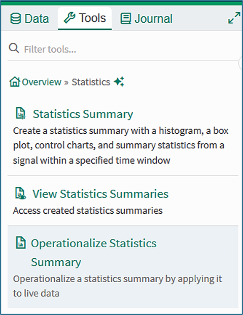
The Operationalize Statistics Summary tool can be opened from the Statistics menu of the Tools pane, or by using the search term Operationalize in the Tools search field. Clicking the tool opens a user interface in the tools pane.
Alternatively, the Operationalize button in the top toolbar of the Summary Report view can be used to operationalize the Statistics Summary that has been selected in the Baseline: field, as shown in Figure 2.
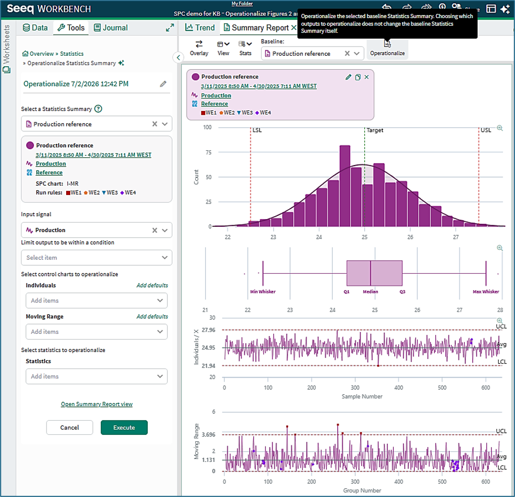
The fields in the User Interface populate automatically with information from the selected baseline Statistics Summary. In the example of Figure 2, the Production Reference Statistics Summary is configured for an I-MR chart with run rules WE1 to WE4.
The fields in the User Interface can be populated or adjusted using the drop-down selectors or by clicking Add defaults.
Using the Operationalize Statistics Summary Tool
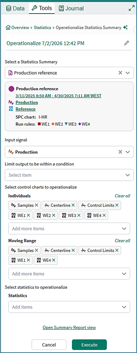
Title: The title field defaults to ‘Operationalize’ plus the date and time. Users can set a custom title for the operationalization instance by editing this field.
Select a Statistics Summary: The selected Statistics Summary will be applied to a signal for continuous monitoring. The selected summary must have been configured with a control chart pair (I-MR, XBar-R, or XBar-S). The configuration is done with the Statistics Summary tool.
Input signal: Normally, the input signal is the same signal that was used to generate the Statistics Summary. It can also be a similar signal, for instance in a second production line.
Limit output to be within a condition (optional): A user can select when to see the monitoring output. For instance, if the Statistics Summary represents operation during manufacture of a particular product grade, the monitoring output should be limited to displaying only when that product grade is being manufactured.
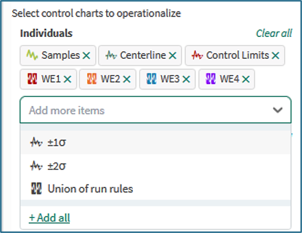
Select control charts to operationalize: The available charts and run rules are those that have been configured in the Statistics Summary. In Figure 3, the Statistics Summary has been configured for I-MR charts with run rules WE1, WE2, WE3, and WE4, where ‘WE’ refers to the Western Electric rules. The I- chart and MR- chart will be displayed in the Seeq Workbench, and violations of the selected run rules will be flagged for automated detection of unwanted process variation.
Figure 3a shows the default selection, while Figure 3b shows other options. Of these, the Union of run rules condition has a capsule when any of the run rules is flagged (i.e. a Boolean OR function on WE1, WE2, WE3 and WE4 in the example of Figure 3a).
Select statistics to operationalize: Selected statistics will be aggregated over each capsule of a periodic condition and displayed in the Seeq Workbench, if they have been configured in the Statistics Summary. Also, statistics that are unavailable or cannot be calculated from the baseline, such as Cpk or Ppk, are omitted rather than displayed as blank. There is more information in a later section of this page.
Open Summary Report View: Clicking this link opens the Summary Report tab in the display pane of the worksheet.
Execute: Clicking the Execute button creates the Operationalization outputs in the Trend view of the worksheet. Any previous outputs that have been subsequently been removed from the tool will also be removed from the Trend and Details panes.
Color coding: The icons for the signal and condition in Figure 3a are grey, while those in Figure 3b are colored. The icons acquire a color when the signal or condition is present in the Details pane of Workbench, typically after the Execute button has been pressed.
Output of a basic I-MR Operationalization run
Details pane
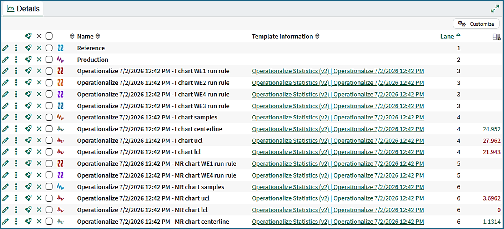
Figure 4 below shows the Details pane where the outputs of the operationalization run from Figure 3 are listed. All outputs are created simultaneously using Seeq Templates and are appropriately grouped together in lanes.
The Template Information column shows the name of the template (Operationalize Statistics) and the specific instance (Operationalize 7/2/2026 12:42 PM) separated by a | symbol.
The right hand column shows the numerical values of the chart limits, which are constant scalar outputs.
Trend view
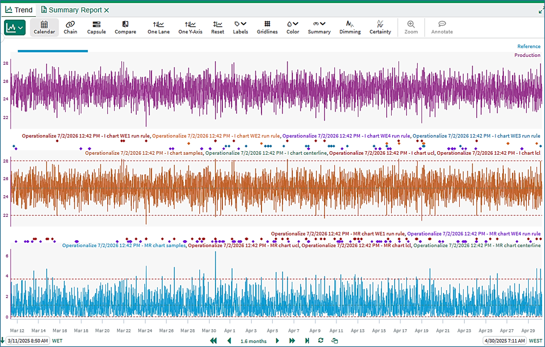
Figure 5 below shows the Trend view where the following can be observed:
Lane 1: The Reference condition under which the Production Reference Statistics Summary was configured. The UCL, LCL and Centerline were calculated from the values of the Production signal under the capsule of the Reference condition;
Lane 2: The Production signal that is being monitored;
Lane 3: Run rule violations for the I-chart marked with point capsules;
Lane 4: The I-chart samples, the I-chart center line, and the upper and lower control limits (UCL and LCL);
Lane 5: Run rule violations for WE1 and WE4 for the MR-chart marked with point capsules. Rules WE2 and WE3 are not used in an MR-chart;
Lane 6: The MR-chart samples, the MR-chart center line, and the upper and lower control limits (UCL and LCL).
Editing an Operationalized Statistics Summary
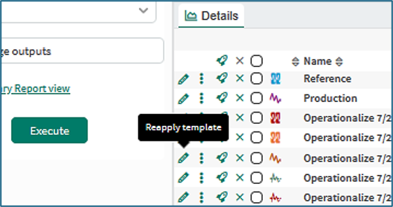
The template instance can be updated and reapplied.
Clicking the Reapply template pencil icon for any of the operationalized signals or scalars in the Details pane will re-open the user interface to allow further editing and adjustment.
The Limit output and Sample alignment conditions
Limit output to a condition
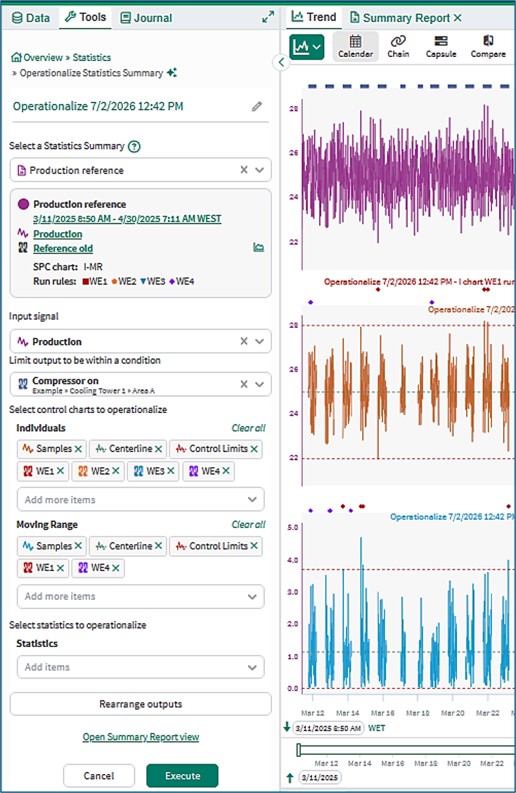
The optional Limit output to be within a condition restricts SPC calculations to measurements collected under specified operating conditions. Measurements outside the capsules of the limiting condition are not displayed. Use cases include:
-
Limiting calculations to production runs
-
Excluding maintenance periods
-
Focusing on particular operating modes or product grades
Figure 7 illustrates the effect of selecting Compressor on as a limiting condition for the Production signal. Compared to Figure 5, the I-chart and MR-chart samples and the run-rule markers are only displayed under the capsules of the Compressor On condition.
Sample alignment Condition
The Sample alignment condition is a mandatory field for the subgroup charts Xbar–R and Xbar–S. A subgroup is a run of several consecutive samples. The average (Xbar) and range (R) or Standards Deviation (S) are calculated for each subgroup. If signal has 1000 samples and a subgroup size of four, there will be around 250 Xbar values.
Sample alignment defines how the subgroup boundaries are determined. The capsules of the Sample alignment condition are operational periods such as shifts, days, batches, or production grades. There must be sufficient samples in each capsule to form subgroups.
Subgroups are anchored to the start of operational periods. In that way, the same subgroups are preserved as the worksheet display pans and zooms.
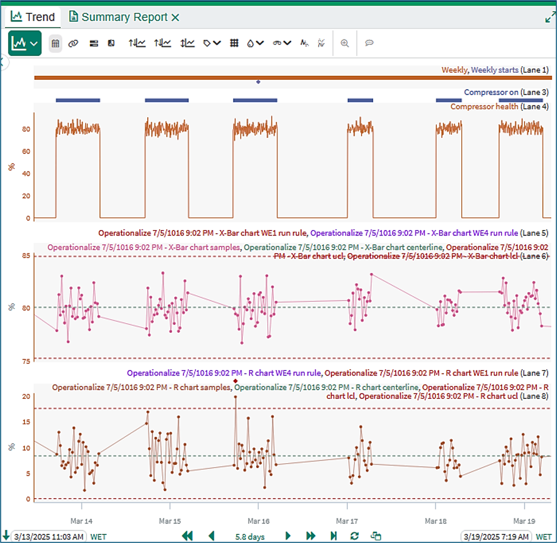
Figure 8 shows the Weekly condition at the top of the worksheet. Included here for the purposes of explanation are point capsules below the brown bar in Lane 1 to mark the start of each Weekly capsule. New subgroups will start at these points.
Inherited values
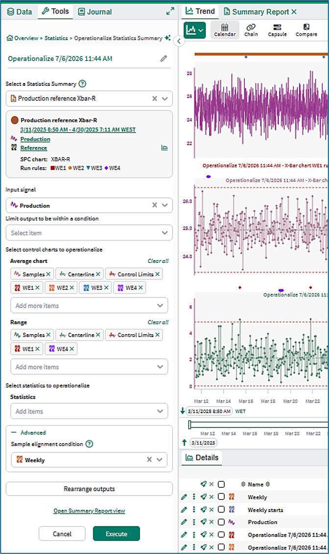
Initially, the Limit output to be within a condition and Sample alignment condition are populated from the baseline Statistics Summary. For example, the Operationalization example in Figure 8 has inherited the default Weekly condition with no limiting of the output from the Production reference Xbar-R Statistics Summary.
Default configuration
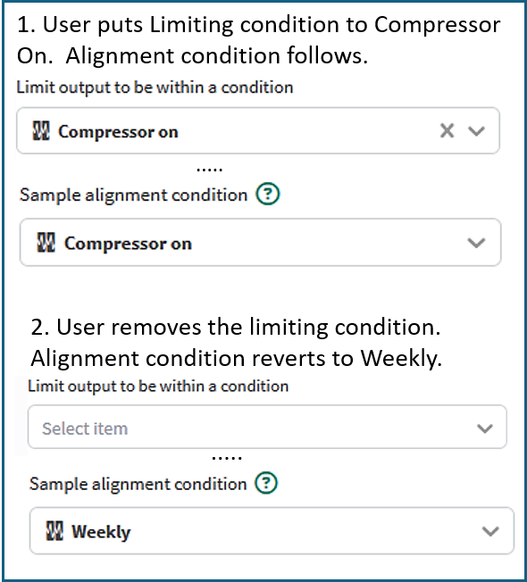
Unless a Sample alignment condition is manually selected, the Sample alignment condition automatically follows the Limiting condition. Changing the Limiting condition updates the alignment condition to match, and removing the Limiting condition reverts the alignment condition to Weekly, as shown in Figure 9a.
Manual configuration
The Sample alignment condition can alternatively be manually configured in the Advanced section of the Operationalize Statistics Summary tool. This is done by means of the pull down menu of the Sample alignment condition field.
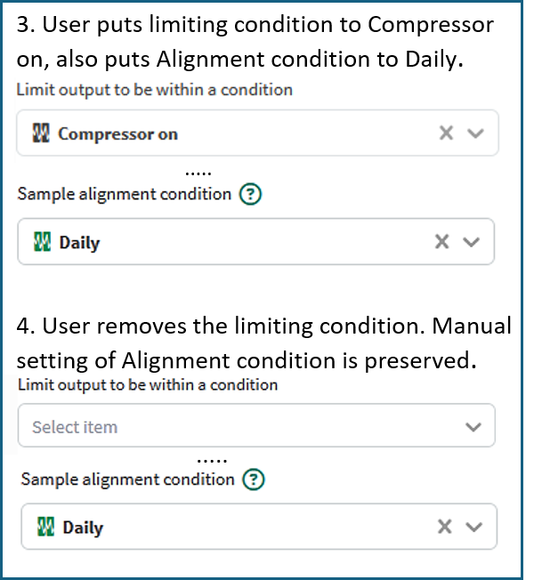
A manual selection is preserved even if the Limiting condition later changes, as shown in Figure 9b.
When a manual selection is active, a clear button ("x") appears on the alignment condition selector. Clicking it clears the manual selection and reverts the alignment condition to the current Limiting condition (or to Weekly if no Limiting condition is selected), after which the alignment condition resumes following the Limiting condition automatically.
Alignment capsule boundaries
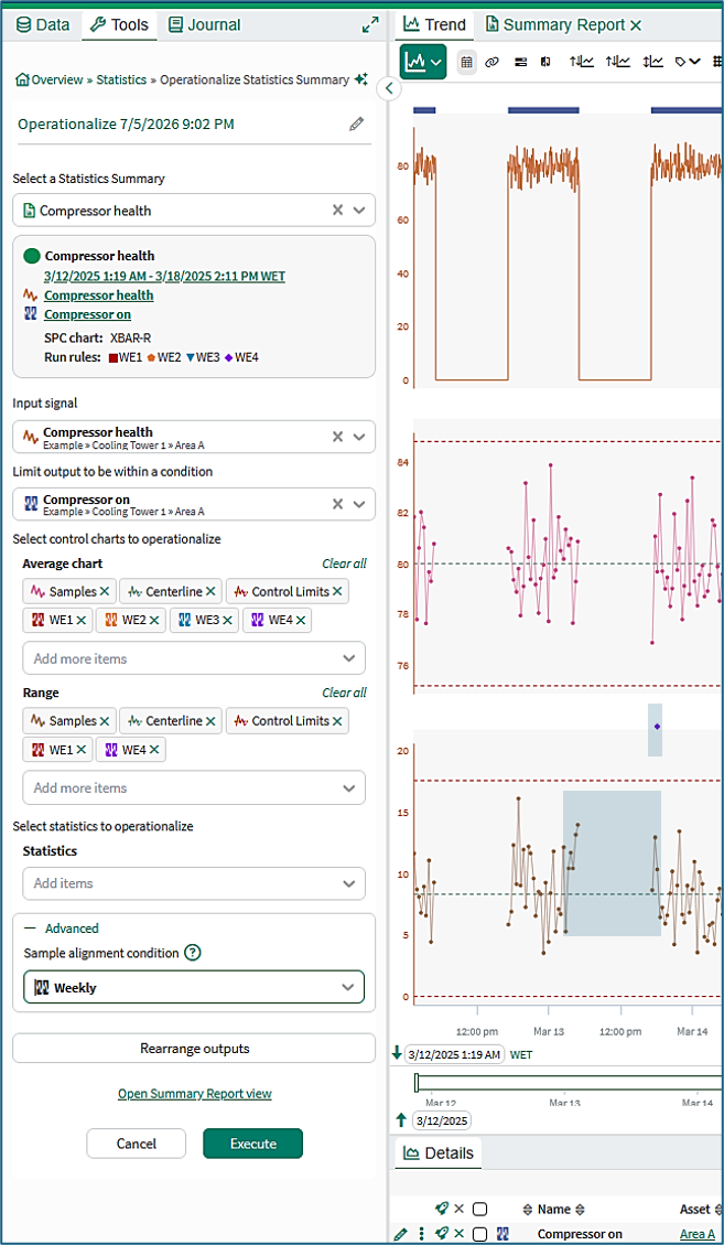
When a new alignment capsule begins, a new subgroup is started and the run rules are reset. There may be a visible gap in the output signal between one alignment capsule and the next, as seen in Figure 10. This happens when the time difference between the final group of the previous capsule and the first group of the next capsule is more than the maximum interpolation of the operationalized signal.
Behavior of subgroups and run rules
Figure 10 illustrates the monitoring of the orange Compressor Health signal in Lane 1 that has measurements only when the compressor is on. Hence, Compressor on is selected as the Limiting condition. The Alignment condition is Weekly.
Subgroups and run rule sequences are reset at the boundaries of Alignment condition.
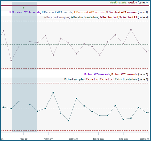
Subgroups and run rule sequences do not reset at the boundaries of Limiting conditions (e.g. Compressor on in Figure 11).
When valid measurements resume in the next capsule of a Limiting condition, subgroup formation and run-rule evaluation continue using the next valid samples unless a sample alignment boundary has been reached.
The right hand side of the shaded area in Figure 11 shows that Western Electric Rule 4 is triggered on the third sample in a capsule of the limiting Compressor on condition. WE4 detects runs where eight consecutive samples are above or below the center line. Here, the WE4 rule has been violated because five sample in the previous capsule of the limiting Compressor On condition were above the center line as well as the three in the right hand capsule of the shaded area.
Unwanted interpolation
Figure 12 shows a situation where the Limiting condition (Weekly) and the Alignment condition (Compressor On) are back to front.
In this case, there may be unwanted interpolation of the SPC chart signals between the capsules of the Compressor On condition. The resolution to this problem is to ensure that the Alignment Condition is a superset of the Limiting condition, for instance Weekly or Daily as shown in Figure 9b, or that it matches the Limiting condition, as shown in Figure 9a.
Statistics Operationalization
Statistics
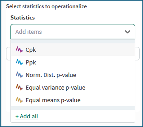
The Statistics section offers the following statistics that can be operationalized. The selected statistics are calculated periodically and displayed in the Trend view of the worksheet.
Capability and performance:
-
Cpk - Process capability index
-
Ppk - Process performance index
-
Normal Distribution p-value
Comparison tests, where the basis for comparison is the Baseline selected for operationalization:
-
Equal Variance p-value
-
Equal Mean p-value
These statistics are described and defined in the Statistics Definitions and Reference page of the Knowledge Base.
Statistics configuration
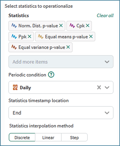
If Statistics are selected, further fields are displayed.
Periodic condition:
Statistics will be calculated within the capsules of the selected periodic condition, for instance, daily, weekly, or monthly. Periodic conditions can be created with the Periodic Condition tool in the Identify tools section in Workbench.
Other conditions with repeating capsules can be selected, for instance to reflect shifts, batches, or product grades.
It will be necessary to specify a maximum capsule duration, if the condition does not already have it.
Statistics timestamp location
The Statistics timestamp location specifies where the timestamp is placed for each calculated statistic value.
Start - Timestamp at the beginning of each capsule
End - Timestamp at the end of each capsule (default)
Duration - The result is displayed across the full time span of each capsule
Statistics interpolation method
The Statistics interpolation method specifies how the calculated statistic values are interpolated between timestamps.
Discrete - Bar chart display with discrete bars (default)
Linear - Line chart with linear interpolation between points
Step - Step interpolation, values hold until the next timestamp
Output of a Statistics Operationalization run
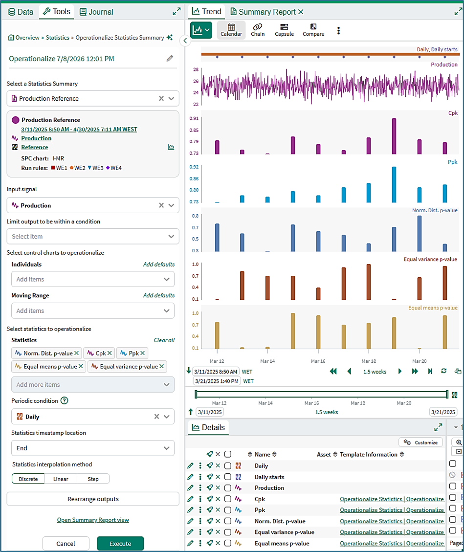
Figure 15 shows the Trend view where the following can be observed:
Lane 1: The periodic Daily condition with the start of each day indicated by a point capsule
Lane 2: The Production signal that is being monitored
Lanes 4 to 7: The operationalized statistics for each day plotted as bars with a timestamp at the end of each day.
The Rearrange outputs function
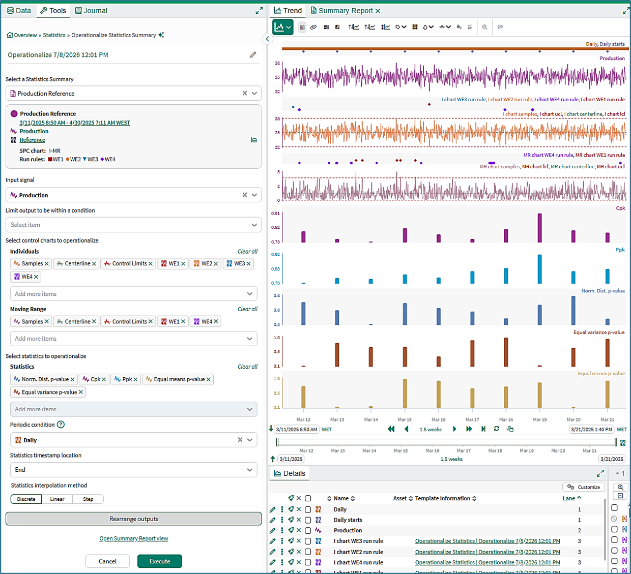
Charts and run rules can be added to the outputs in Figure 15 by clicking a pencil icon beside any one of the items in the Details pane, then editing the Operationalization tool, and then clicking Execute. However, the charts will be added at the bottom of the trend view.
Clicking the Rearrange outputs button resets the Trend view to its canonical layout with run rules above charts, and statistics grouped at the bottom of the trend in designated lanes, as illustrated in Figure 16.
The Rearrange outputs button can also be used after a manual rearrangement, to reset the display to its canonical layout.
Further information
Information is available in the Statistics Summary KB on the topics of:
-
Opening the Statistics Summary tool
-
Using the Statistics Summary tool
-
Content of a basic Statistics Summary
-
Content of a Statistics Summary with SPC Chart
-
SPC Chart types
-
SPC Chart limits
-
SPC run rules
-
The Limit and Sample Alignment conditions
Information is available in the View Statistics Summaries KB on the topics of:
-
Opening the View Statistics Summaries tool
-
Using the View Statistics Summaries Tool
-
Summary Report
Information is available in the Summary Report KB on the topics of:
-
Opening a Summary Report
-
Tabbed viewing
-
Summary Report controls and configuration
-
Working with multiple statistics summaries
-
Quantitative comparisons
Information is available in the Statistics Definitions and Reference KB on the topics of:
-
Contents of the Statistics table
-
Box plot calculations
-
Performance calculations
-
Probability calculations
-
Autocorrelation and discrete signals