Interpolation
Overview
Interpolation deals with how samples are connected. Here we'll discuss the different options for it, their impact on calculations, as well as how to discover and set interpolation for your signals.
Interpolation Method
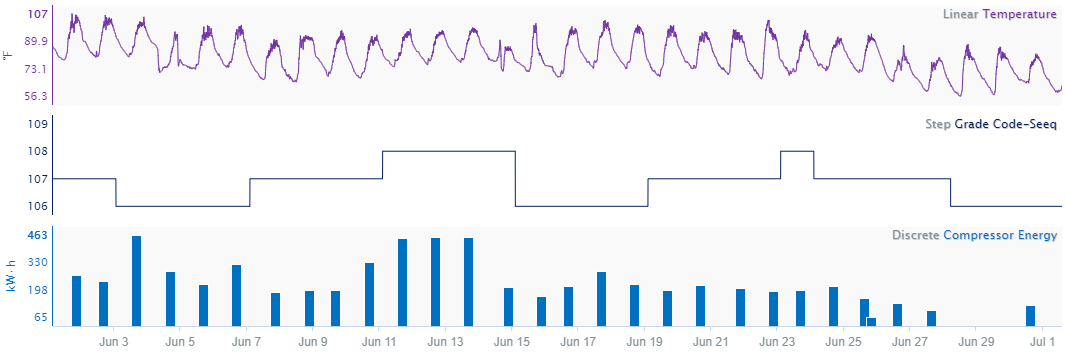
Interpolation deals with how are samples connected since samples only occur at select timestamps. Some datasources allow users to designate how their tags are interpolated. We are able to bring this information into Seeq. In order for Seeq to perform calculations across different signals with different sample times, interpolation is needed to infer what would the value of a signal be at a point in time where there is not a sample. There are four types of interpolation - Linear, Step, Pi Linear and Discrete. Each of these can result in different inferred values between samples so it is important to know which interpolation method is being used.
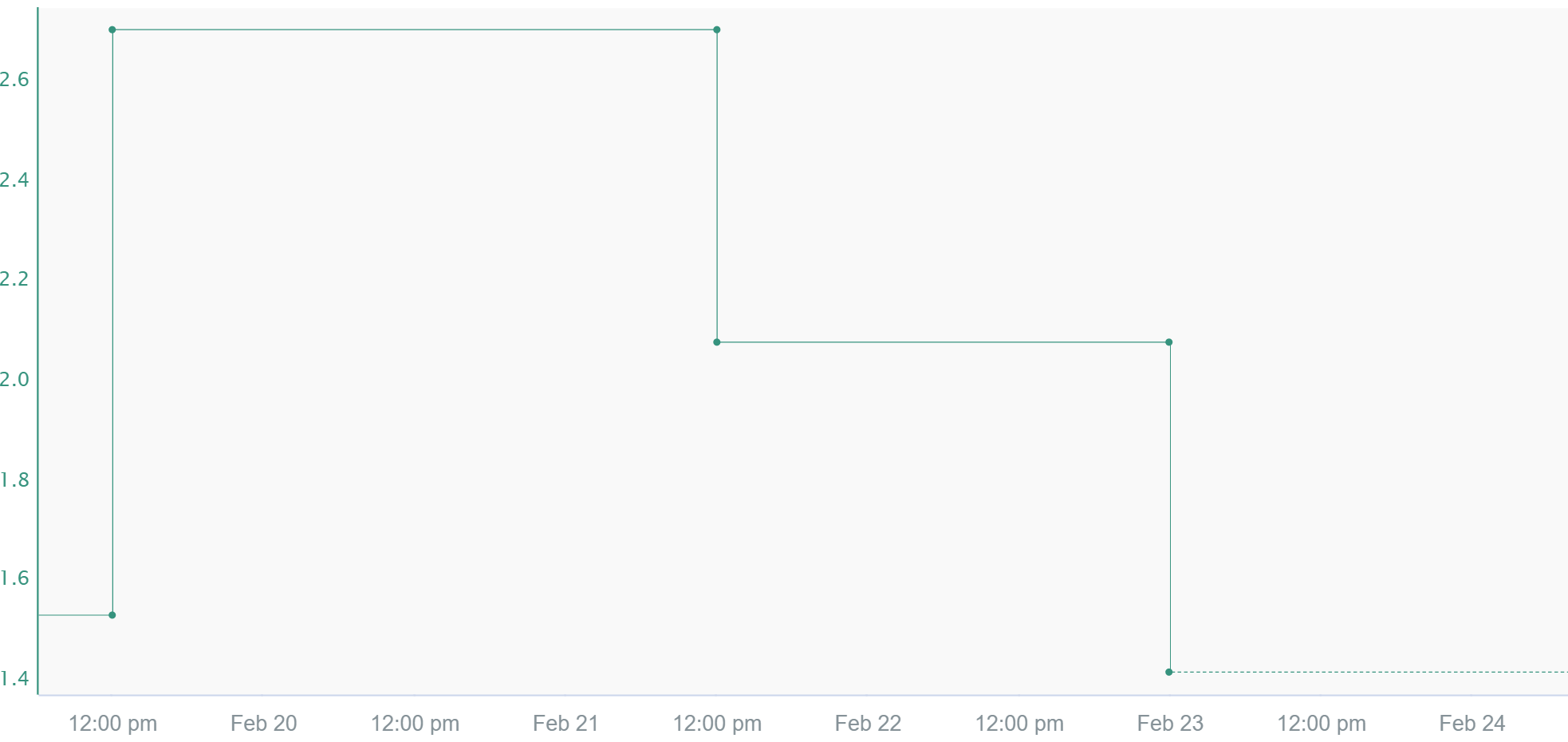
Step
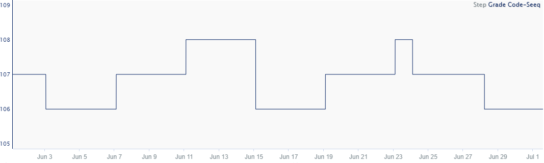
The value of a signal stays equal to the value at its previous sample until a new sample appears. In Seeq, we are able to use step interpolation by inserting a proxy sample to serve as the start of the step. This additional sample becomes important when calculating running sums where each individual sample matters. Step interpolation also plays a role when calculating derivatives. Due to the immediate steps, near infinite derivatives are calculated when determining the derivative for step signals. Lastly, step interpolated signals project the last sample's value to now if the time elapsed since this sample occurred is equal to or less than the maximum interpolation. More information about the maximum interpolation is shown below. Typically, tags coming from LIMS are step interpolated since for most processes, an overall decline/increase to the next sample point isn't likely.
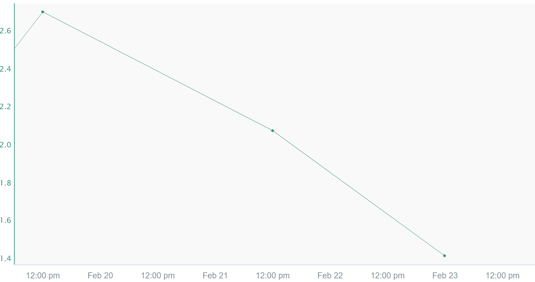
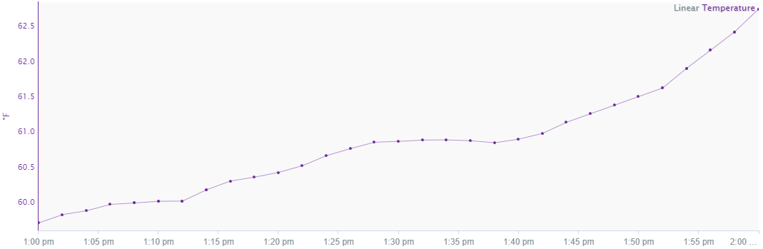
Linear
The value of the signal in between two samples is the linear interpolation between them. The calculation to determine this value is done by first finding the rate of change between the two samples. This number is then multiplied by the difference in time between the previous sample and the timestamp being looked at. Finally, this number is added to the previous sample's value. When calculating derivatives or running sums, this is the preferred interpolation method. Linear interpolation tend to be used in process data where it makes sense that a gradual increase/decrease occurred rather than an instantaeous change.
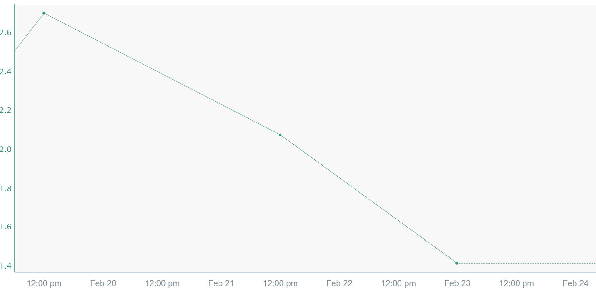
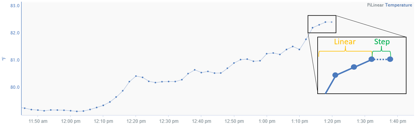
Pi Linear
This interpolation method is similar to Linear except whenever there is not a new sample yet. In this situation, it behaves like Step interpolation and projects the last known value based on the signal's sampling rate. This interpolation method is typically seen in data coming from OSIsoft products (PI Data Archive, Asset Framework) but can be applied to any signal in Seeq.
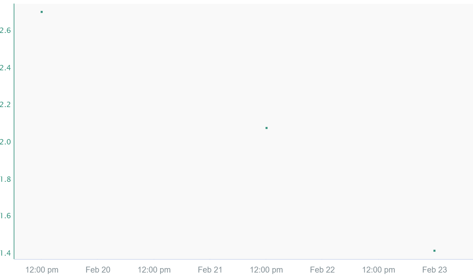
Discrete
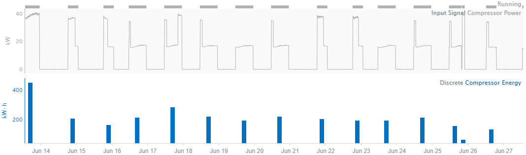
Only exact samples are shown. This interpolation method produces a discontinuous signal with gaps of invalid values between samples. As a result, if calculations are used with discrete signals, there will only be values exactly at the timestamps of the discrete signals if they happen to align. Since Discrete interpolation only shows samples, it can be difficult to place a cursor on the sample to see what values are there. Customizing the signal to trend as a bar graph makes it easier to discover the values of the samples.
Determining the Appropriate Interpolation Type
Linear
Data measuring a quantity that is changing continuously. For instance, temperature data are usually continuous (i.e. measuring temperature in a given environment as that environment changes continuously): if the temperature measured by a given sensor is 10 C at one time and 20 C a short time later, the temperature can usually be assumed to be between 10 C and 20 C between these time points. With linear interpolation, the change in temperature between two data points is assumed to be linear.
Step
Data measuring a quantity that holds constant until a new sample is obtained. For instance, a unit produces either Product A or Product B. When production of Product A begins, the product code is set to Product A and holds steady until the process changes to Product B. When the process changes, there is an abrupt change from A to B. In this case, it may be most appropriate to view this transition as a step change to the new product. Note that every time value has a data value.
Discrete
Data measuring a quantity, such an aggregated quantity, that is not dependent on earlier values, does not influence later values, and does not change continuously. For example, data measuring the amount of energy used for a batch process is discrete: the measured value of the metric does not change continuously between batches because each batch can be considered a different population. For instance, one day, the process uses 1000 kWh of energy. On the next batch, 900 kWh is used. There is no continuous change from the first energy value to the second, in other words, the the energy use is not 950 kWh between the two batches, as linear interpolation may suggest. Each batch has a unique value, unrelated to the previous, so the data points are not connected.
Additionally, discrete data points do not have definitive time stamps because each one is calculated over a range of time. For example, when quantifying the amount of energy used by a compressor during a day, one could choose to display the value at midnight of the day being measured, in the middle of the day at noon, or at the end of the day. All display options are technically correct because the discrete data are not unique to a single hour or minute: the user must choose how to display the data as appropriate for visual purposes and subsequent calculations. Each display option has its own benefits depending the analysis being performed. Note that because of the ambiguity of the chosen time stamp, discrete data points should not be connected linearly. For example, displaying the data at the beginning of each day, versus the end of the day, can produce significantly different results for a linearly interpolated value between the two points. Step interpolation may not be appropriate either if the calculated data is not holding constant across time until a new sample is obtained.
Pi Linear
Data that are interpolated using a hybrid of Linear and Step. Pi Linear (i.e. in aggregate() in Formula) uses linear interpolation between data points except when there is no “next” data point to connect to. When there is no new data point, Pi Linear uses Step interpolation to project the last known value into the future based on the signal's sampling rate. Pi Linear interpolation is typically seen in data coming from OSIsoft products (PI Data Archive, Asset Framework) but can be applied to any signal in Seeq.
Usage in Seeq
Maximum Interpolation
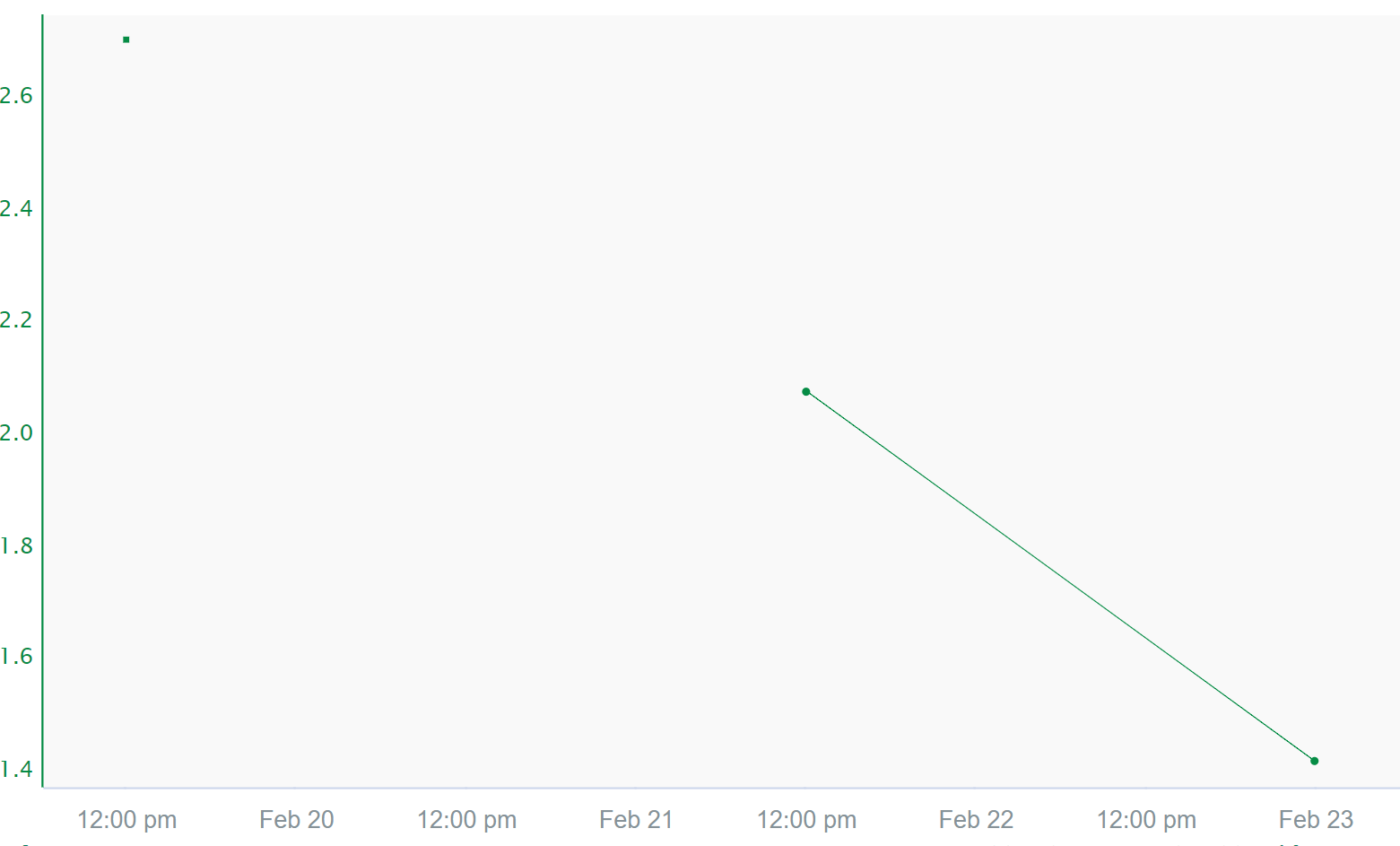
Maximum interpolation deals with the maximum amount of time two samples will be connected, independent of which interpolation method is used. If two points happen to be spaced apart more than the maximum interpolation, interpolation will not occur and a gap will appear between the two samples. In the example below, the signal has a maximum interpolation of 40 hours. The two connected samples happen to be 36 hours apart whereas the samples that are not connected are separated by 48 hours, more than the 40 hour maximum interpolation.
Signal From Condition
Signal From Condition is a tool used to perform aggregations during conditions. More information about the tool can be found at Signal from Condition. The same interpolation options mentioned above are available but additional considerations have to be made since this tool also gives the ability to select where samples are placed. Different combinations of sample placement and interpolation yield different results that can be misleading. A common misleading example is seen when placing the sample at the End of the capsule in Signal From Condition, and using step interpolation. This results in a value based on previous capsule being carried over the next capsule. Some users tend to associate the value of a signal with the capsule it overlaps with, which in this case would be incorrect.
Identifying and Changing Interpolation
Item Properties
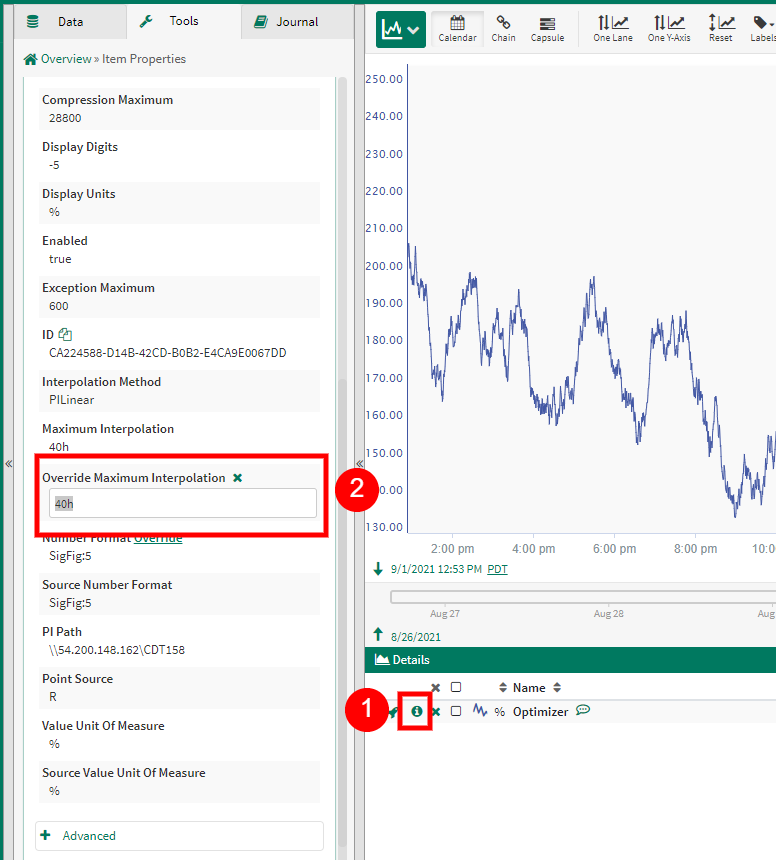
In order to find out the interpolation method and maximum interpolation associated with a signal, look at the item properties of the signal. More information can be found at Item Properties.
Users with read/write permissions to a signal can change the maximum interpolation of signals directly from connected datasources through the item properties panel. This which will change the max interpolation value for all calculations on the server that reference this signal. Changing the default interpolation method for every signal on a server can either be done in the source historian/database or by adding a Connector Property Transform. Default interpolation methods cant be changed in the Item Properties panel.
Formula
In the case that you'd like to change the interpolation of a signal, admin users or users with write access to a signal are able to override the maximum interpolation in the Item Properties. These changes are carried over the Seeq server so that every user would see the same maximum interpolation. For regular users and in cases where this change would not want to be propagated across the server, the Formula tool can be used to edit the interpolation method and maximum interpolation of an alias. In order to change the method, use the function .toStep(), .toLinear(), .toPiLinear() or .toDiscrete() to change the signal to Step, Linear, Pi Linear or Discrete. These functions also take the maximum interpolation as parameters such that .toLinear(3d) changes the interpolation to Linear and also changes the maximum interpolation to 3 days. In the case that you'd want to keep the same interpolation method and only change the maximum interpolation, the .setMaxInterpolation() function should be used.
FAQ: Why is my trend not connecting between two points?
If you see a “break” (gap) between two samples that you expect to be connected, it’s usually one of these:
there’s an invalid value somewhere between those points, or
the time gap between samples exceeds the signal’s Maximum Interpolation setting.
Cause 1: There’s an invalid value between the two points
What’s happening
Even if you can see two “good” samples on either side, a single invalid sample in between can prevent Seeq from drawing a continuous trend (because the signal is not considered valid across that interval).
How to fix it (analysis-side / local fix)
If you’re okay treating invalid samples as “ignore and continue,” you can filter them out in Formula:
Use
validValues()to drop invalid values and allow interpolation to connect across the remaining valid samples.
Example:
$signal.validValues()When to use validValues()
Use this when you accept a bit of ambiguity: you’re choosing to ignore bad/uncertain points rather than diagnose why they were logged as invalid. If your analysis requires full accuracy (e.g., auditing, compliance, custody transfer, or anything where missing/invalid points must be explained), you should investigate the source of invalidity instead of filtering it away.
If the underlying issue was fixed in the datasource
If the invalid values were corrected upstream (historian/database) and you still see gaps, the trend may be reflecting cached results. In that case:
Clear the cache for that item, then re-check the trend.
After cache clear, the line should connect without needingvalidValues()(assuming the data is now valid).
Cause 2: The sample gap exceeds Maximum Interpolation
What’s happening
Maximum Interpolation sets the largest time span over which Seeq will connect samples (regardless of interpolation method). If two consecutive samples are farther apart than this threshold, Seeq will show a gap instead of connecting them.
How to fix it (pick the scope you want)
Option A — Local fix (only affects your formula/alias)
If you just want your analysis to connect across larger gaps, override it in Formula:
$signal.setMaxInterpolation(1h)(Use a value appropriate for your use case/data: 10m, 1h, 3d, etc.)
Option B — Change the item’s Maximum Interpolation (affects everyone)
If you have write access, you can update Maximum Interpolation in the Item Properties panel.
This changes how the signal behaves for all calculations on the server that reference that signal.
Option C — Change the default at the datasource level
If many signals from the same datasource need a different Maximum Interpolation, a datasource admin can apply a Connector Property Transform to set it for all (or a subset of) signals during indexing.
Quick Troubleshooting Checklist
In Workbench Zoom in and see whether there are any or gaps between samples that are less than the maximum interpolation.
Check Item Properties > Maximum Interpolation and compare it to the actual time gap between the two samples.
If data was fixed upstream but Seeq still shows the old behavior, clear the item cache.