Prediction
Prediction enables users to predict a signal based on other correlated signals with linear and non-linear regression models.
Using the Prediction Tool
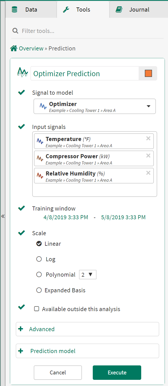
Signal to model: From the dropdown menu, select the signal to model from the details pane, pinned items or recently accessed sections.
Input signals: From the dropdown menu, select at least one signal to serve as independent variable(s) for the regression model.
Training window: Select the fixed window of data on which the regression model will be based.
Options: Select the type of regression between Linear, Log, Polynomial (2nd to 9th degree) and Expanded Basis (called Automatic before R20.0.38.00). The Expanded Basis option applies a combination of linear, 2nd and 3rd polynomials and cross-products.
Available outside this analysis: Checking this box will allow this condition to be used in other workbench analysis and topics. It will be available for all Seeq users and will display in their search results. Consider using a unique name as the signal will be published to the global name space.
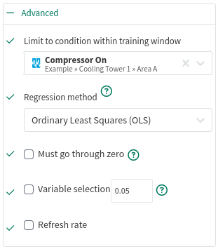
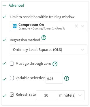
Advanced Options:
Limit to condition within training window: You can choose to limit the regression only to the data from within the training window and within a condition. For example, choose a condition that identifies when an operation is running and all data outside of the condition (when the unit is not running) will be ignored for the regression analysis.
Regression method: You can choose from one of several different regression algorithms:
Ordinary Least Squares (OLS) can safely be used for most predictions. It calculates a linear regression by minimizing standard error with respect to the target signal. OLS's main disadvantage is that is does not correct for multicollinearity (where one input can be predicted from another input). In most cases, this is fine because the output still provides an accurate linear model. It becomes problematic in if one wishes to use some of the coefficients from the model individually rather than all of them together.
Must go through zero: You can choose to force the regression to go through zero or the origin (0, 0). This may be used if you are reasonably certain the data you are modeling fits the selected scale and that the target truly is zero when all the inputs are zero (E.G. units produced based on conveyor belt speed). The Sum of Squares statistics are zero-based rather than average-based when this option is used, therefore the R-Squared value is not comparable to the R-Squared of other options.
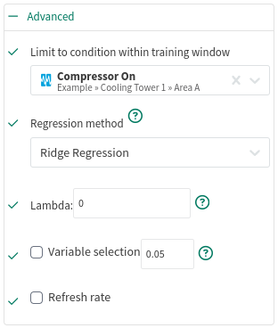
Ridge Regression is one way to reduce issues from collinearity. Ridge includes a basis factor to scale some coefficients toward 0. The coefficients which are scaled are those which have less of an influence on the dependent variable.
Lambda: The bias-variance trade-off tuning parameter. Values are typically between 0 and 1, but can approach infinity. The higher the lambda, the more strongly the coefficients will get scaled toward 0. A non-zero value is generally inadvisable unless you are dealing with issues from multicollinearity.
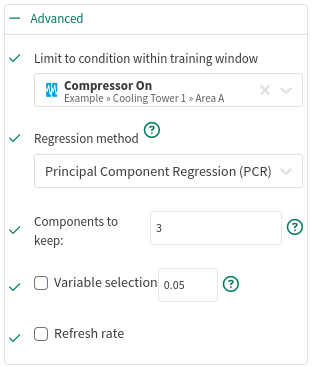
Principal Component Analysis (PCA) approaches the collinearity differently. Each of the (possibly collinear) input signals will be transformed into a set of (uncorrelated) principal components and are ranked. The worst n components are ignored. After this removal, the regression itself is performed.
Components to Keep: Keep between 1 and the number of input components. Components are not necessarily the same as an input signal, but are linearly uncorrelated variables calculated from those input signals.
Variable selection: You can choose to filter away coefficients with P-values that are higher than the provided number. The P-value tests the impact of the "null hypothesis" for each coefficient. Values approaching 0 indicate that the data contributes significantly the model; values approaching 1 indicate that the contribution could be attributed to random noise. Coefficients with a P-value of 0.05 or less are generally considered "statistically significant" for predictions.
Refresh Rate: You can choose to limit the recalculation of the prediction model to increase Seeq performance. The model will be recalculated at most once per the specified duration. Refresh Rate temporarily caches the model’s coefficients in memory until the configured time expires. This is especially useful when prediction models are trained with a changing dataset. Although new datums may be recorded frequently, this tool prevents the model from recalculating every time data become available.
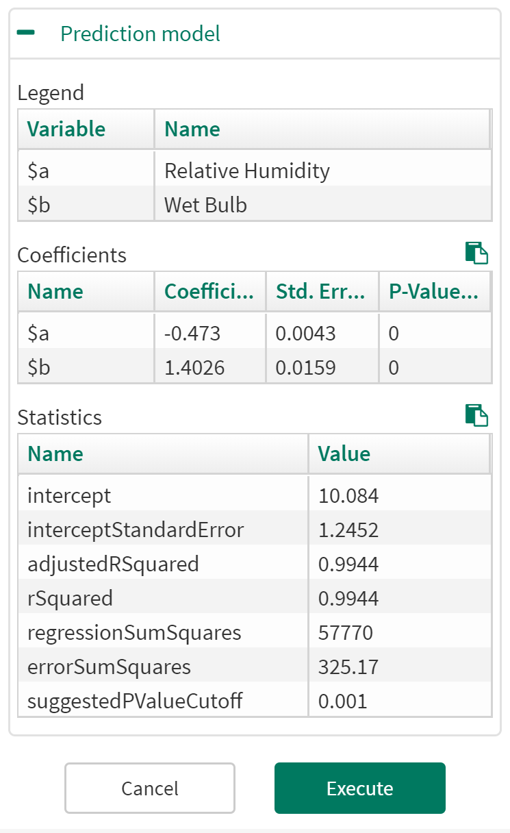
Prediction Model: You can view the Legend, Coefficients and Statistics for the resulting prediction model. You can also change the model type in "Options" and observe how the prediction model results change within the tool. Any single input Predictions can be displayed on a XY Plot.
The adjusted R Squared can also be viewed alongside the standard R Squared calculation. The adjusted R squared value takes into account the number of independent variables used in the model. Use the adjusted R squared to better compare Prediction models with a different number of input variables.
Get the model equation by looking at the Coefficients table: multiply each "$_" variable in the Name column by the associated Coefficient value, add all the equation terms together (one term for each row in the Coefficients table), and then add the Intercept from the Statistics Table.
In this picture, the model equation would be:
y = (-0.473*$a) + (1.4026*$b) + 10.084