Best Practices for using forecastArima

Arima forecasting for time series data can be highly valueable, however it is not as plug and play as some of the other time series operations that can be accomplished in Seeq.

Lets start with best practices, if you are interested in learning more about ARIMA modeling and how it was implemented in Seeq, find that below the Best Practices.

📘 Best Practices When Using forecastArima() in Seeq Formula

To explore best practices, the Example >> Area A (and C) >> Temperature signal will be used which does not show a longer term rise or fall. The goal for my model was to develop a forecast that predicts the daily temperature swings (seasonality). Depending on the goals of your model, you may need to deviate from these suggestions to get the results that best suit your usecase.

Use Clean Data: Clean your data as needed. As with all models, the more we can remove noise or bad data, the better the model results will be. If you dont remove bad data, your model will assume that is part of what needs to be forecasted like in the following example using Area C Temperature in the example dataset:
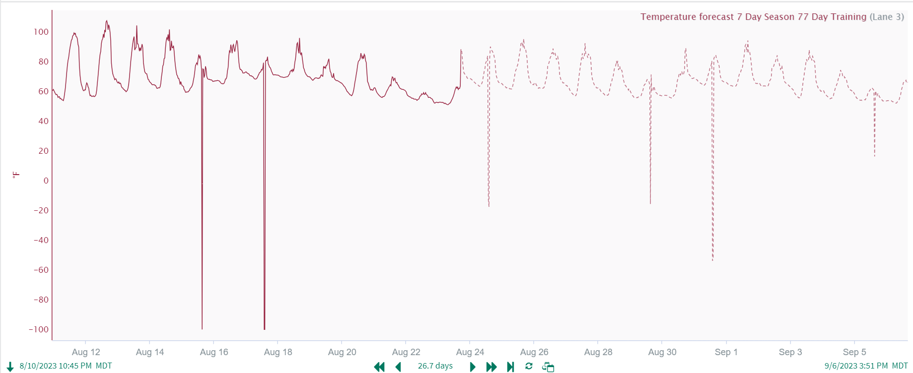
Note: Without removing bad data, I had to expand the Training Window to 11X my season in order to get a reasonable result. With noisy data, you might require a longer training interval to get the model you are looking for.
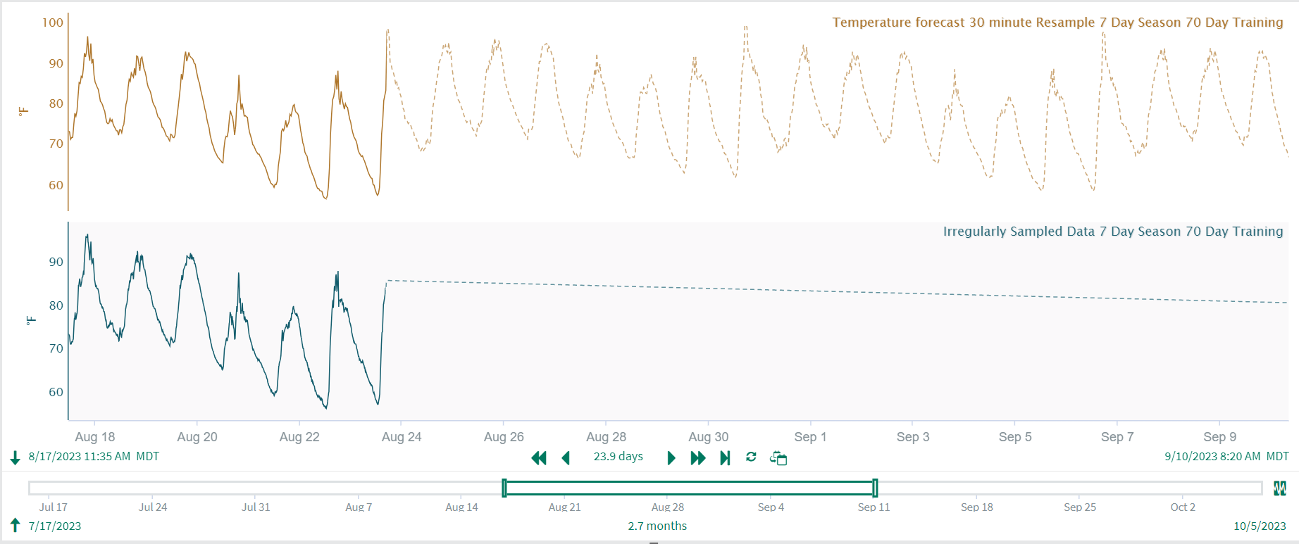
Resample your data to a standard interval. Because ARIMA models use Auto-regressive and moving average terms, they perform best on downsampled data at a consistent interval. Depending on the desired output and model it is best to downsample your data to a 30 minute to 6 hour interval, or to calculate some metric to run the model on i.e. daily average/max value.
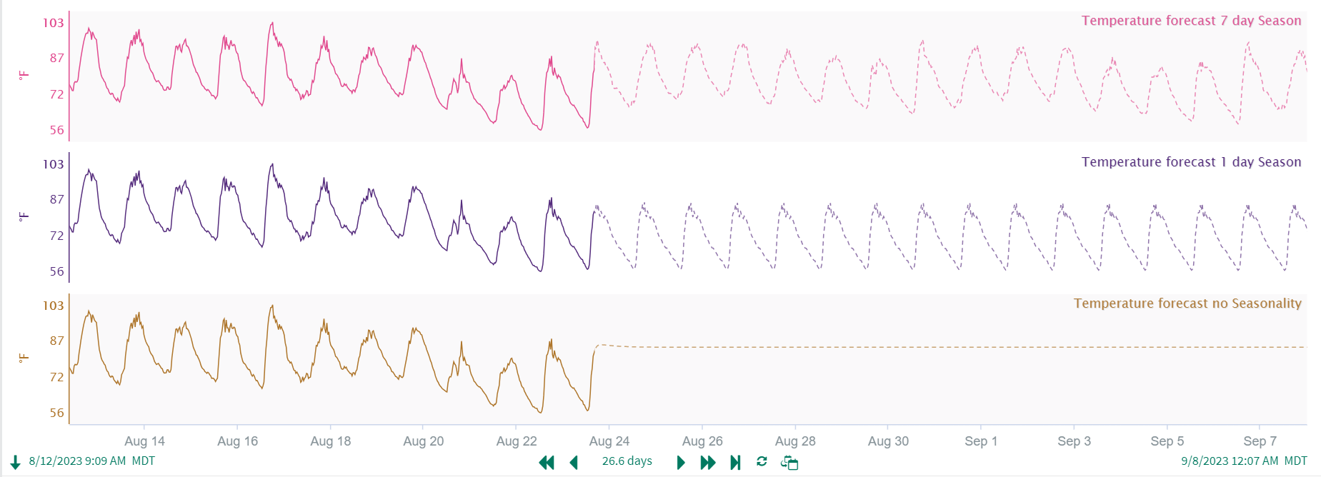
Determine if your data has a ‘Seasonal’ component. This is typically the duration of the cycle you expect to see, but it might help to experiment a bit with your seasonality. I.e. if we are looking at temperature recorded on an hourly interval, I might try a seasonal duration of 1 day, 7 days, etc. Here, you can see an example of how seasonality affects the model when everything else is held constant. Note that the 7 day seasonality shows day to day variation whereas the 1 day seasonality shows a consistent forecast for the day.
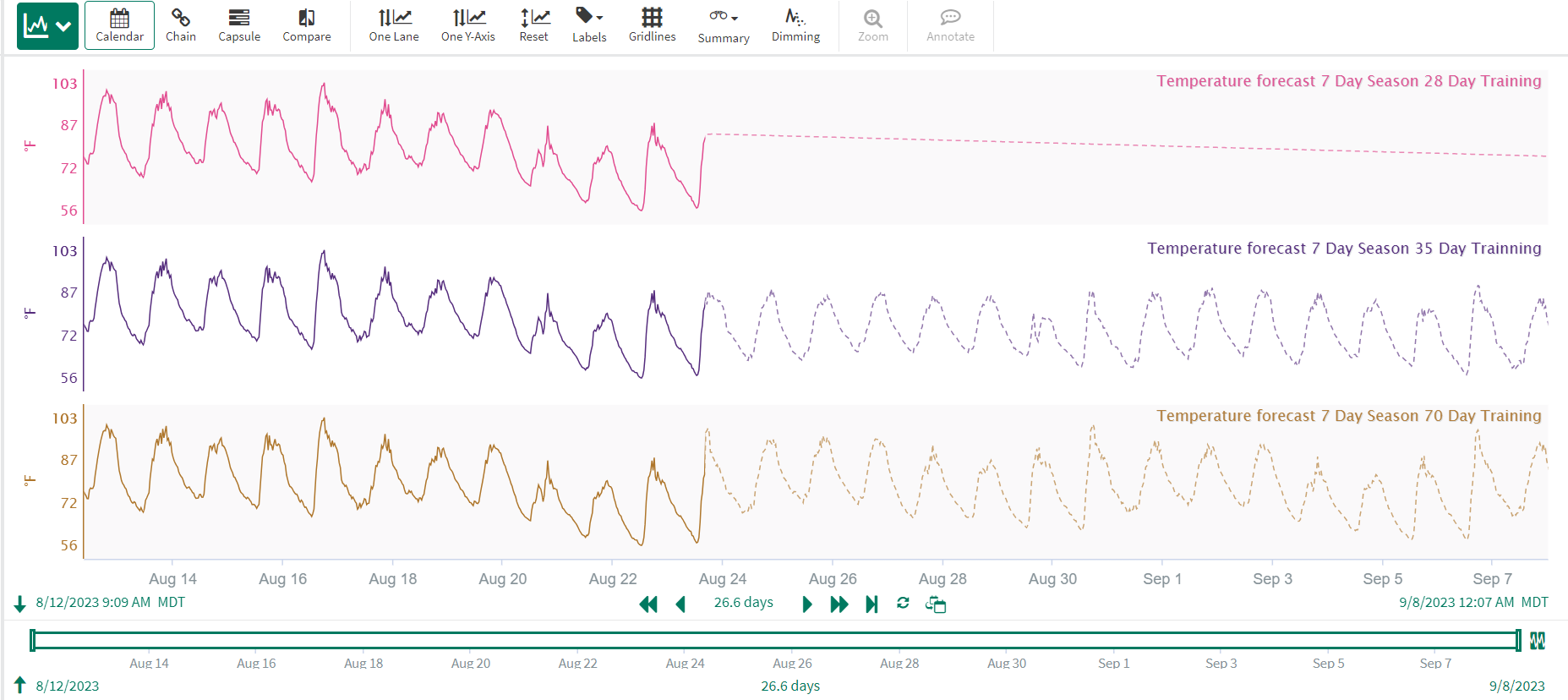
Find your training window. (S)ARIMA models can require a large training dataset to properly capture seasonality if present. If you have a seasonal component in your data, try to include at least 5 seasons in your training dataset, but 7 or so might be a bit better. Any fewer than 4 seasons in your training window will likely result in a model that does not meet expectations. This will likely be a tradeoff between model accuracy and performance. The more you downsample your data, the longer the window you can include in your training period without sacrificing performance. In general, you don't need more than ~10 or so seasons to adequately capture variation. As an example, if my “season” for my temperature data is 1 day, I should try to include about 7 days of data in my training window. If instead, my season is 7 days, I should aim for at least 35 days (7*5=35) in my training data, but 49-70 days (7 to 10 seasons at 7 days per season) might give a better output. In the below example, you can see a training window of 4X the season duration does not give a good forecast, while even a 5X Season gives a realistic forecast. A 10X Season for the training window seems to do a better job of capturing variation but offers minimal improvement over the 5X Season training duration.
Develop Upper and Lower Confidence Intervals (if needed). The forecastArima() function allows the user to also create upper and lower confidence intervals to forecast a range of data rather than just one trend. By creating an upper and lower signal as well, you can better convey the range of expected values to subsequent users. To do this, supply ‘upper’ or ‘lower’ in your formula. When combining all three signals using the Scorecard Metric, you get a forecast with an expected range:
CODE
```
$signal.resample(30min).forecastArima(49d, 30d, 7d, 'upper')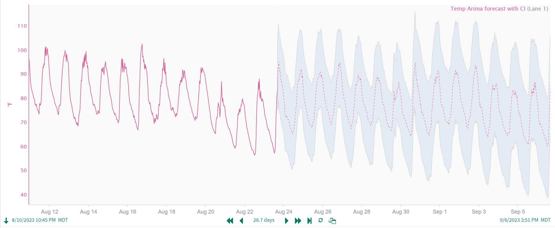
```

Troubleshooting

What happens if my model seems to converge on a single value or shoot off towards infinity?

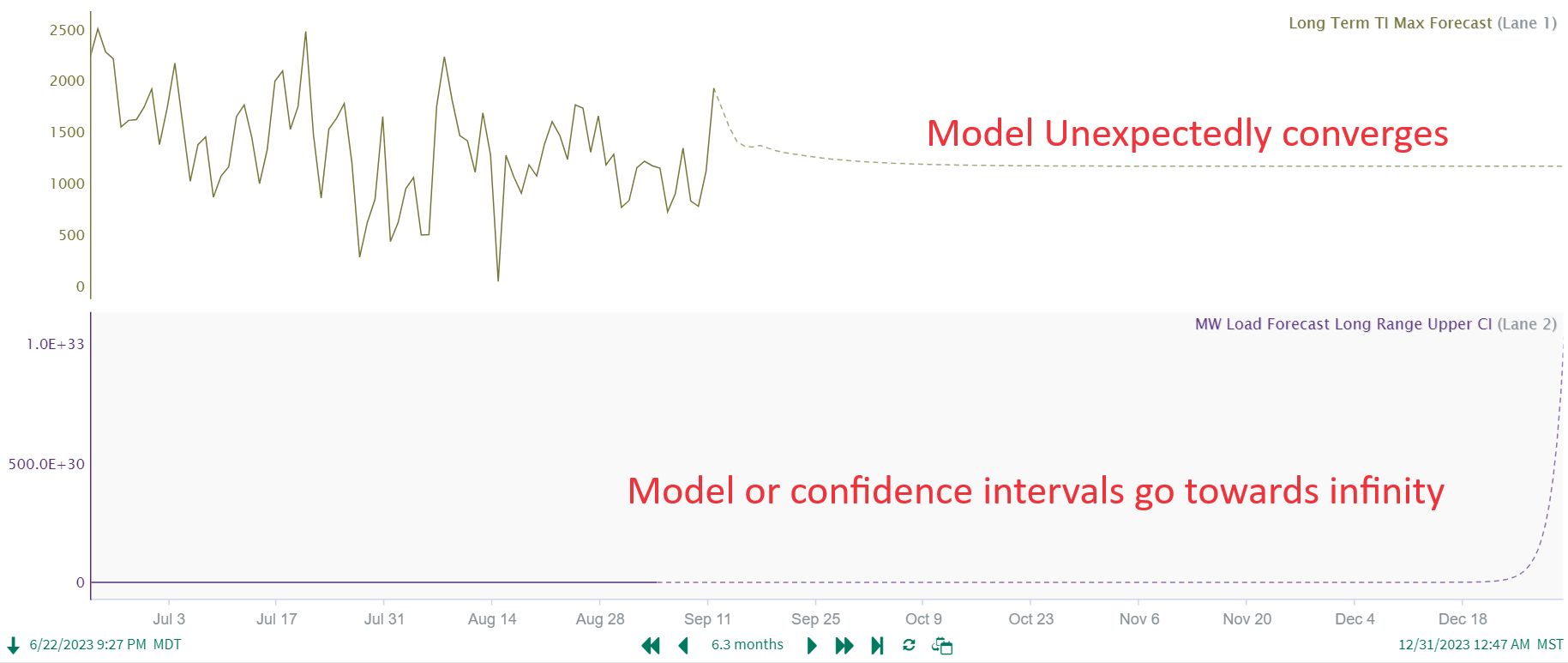
This is more likely while using the upper or lower confidence intervals, but can happen with a model as well. This usually indicates that your model has low confidence (even though the model itself might look really good!) or the model or input data need to be tuned if you are expecting to see different results.

Try:

Adjusting your seasonality- your model might not have a strong seasonality to it resulting in low confidence and wide confidence intervals, try getting rid of the seasonality in the model for the confidence intervals.
Adjusting your training period- you might not have enough seasons in your training window to get a better model. Try expanding the training window to include more seasons if possible.
Adjusting your input data- There might be too much variability (noise) in the input data to build a good or high confidence model, try downsampling or filtering your input data (or increase the downsample/filtering if you are already doing this)

About ARIMA Modeling

What is an ARIMA Model?

ARIMA stands for: Auto Regressive Integrated Moving Average, in other words, an ARIMA model combines auto regressive (AR), differencing/Integrated (I), and moving average (MA) components into a single univariate model, each with its own term, with an optional seasonality component (S). This means that an (S)ARIMA model will use past variability and signal trajectory as well as a seasonal component to project the value of a signal out into the future. Here is a more in-depth description of the math behind ARIMA models on Wikipedia.

Arima Models are seen as a general enhancement for time series forecasting in terms of modeling variability (especially seasonality in signals that have a seasonal component) in a signal as it is projected forward in time over something like a linear model. Using the example of temperature, if I forecast a linear model I will either: forecast the average value of the temperature for a day if I use a long history, or project the trajectory of the temperature forward (which will quickly result in unrealistic values) if using a few hours to train my model. By implementing an (S)ARIMA model, my model will capture the daily rise and fall and will create a forecast that includes this daily rise and fall. It is very important to remember that (S)ARIMA models do not take into account any first principles to project values forward, but instead use the signal trajectory and the Autoregressive, Differencing, and Moving Average components to create a forecast.

Seasonality In ARIMA

When discussing ARIMA models (technically (S)ARIMA models when seasonality is included), seasonality does not necessarily reference the seasons (spring, summer, fall, winter) but rather is in reference to something that might happen in a cyclic fashion over and over again, like the seasons that happen each year. A great example of this is the daily rise and fall in temperature over the course of a day, which can be said to have a “seasonality” component of 1 day if we are looking to capture that daily rise and fall. Alternatively, if I am looking at only the daily Maximum Temperature, I might instead adjust my seasonality to be something like 4 months or 1 year to account for the temperature swing in daily maximum temperatures over the course of the year.

Stationarity

In general, it is best practice to check for stationarity and seasonality in your data prior to using an ARIMA model. We already discussed seasonality, which in the case of (S)ARIMA models is the period over which we can expect the trend to repeat. Stationarity means that the data does not have a trend over time i.e. the trend-line is flat if I draw a trend-line through the dataset over time. For many datasets, however, this likely wont be the case. Often the point of forecasting something forward in time for process data is to understand when it might cross a threshold. This is where the “I" term comes in. (S)ARIMA models implemented in Seeq can handle up to a 1st order integration. If your data is increasing/decreasing logrithmically, exponentially, or follows some other curve over time, it is best to account for this before using an (S)ARIMA model to get accurate results, i.e. if you have a function that is exponentially increasing, try taking a logarithm of the data to linearize.

ARIMA as implemented in Seeq Formula

When using forecastArima() in Seeq, rather than specifying each of the ARIMA components, Seeq implements an Auto-ARIMA algorithm to determine the best orders for each of the Autoregressive, Integrated (or differencing) and Moving Average components for the model. This is similar to how many Arima models are developed in Python. If you need to use a higher order of differencing, or would like to manually specify some of your model parameters, this is best accomplished using Seeq Data Lab.