Use Case Walk-Through

In this simple walk through, we will guide you how to utilize Scaling Tables to deploy time-series analytics across the fleet of “Example” Compressors that are shipped with every Seeq system. Although this use case only performs calculations for 11 assets, this same metholody can be used when you have thousands!

Step 1: Define your search

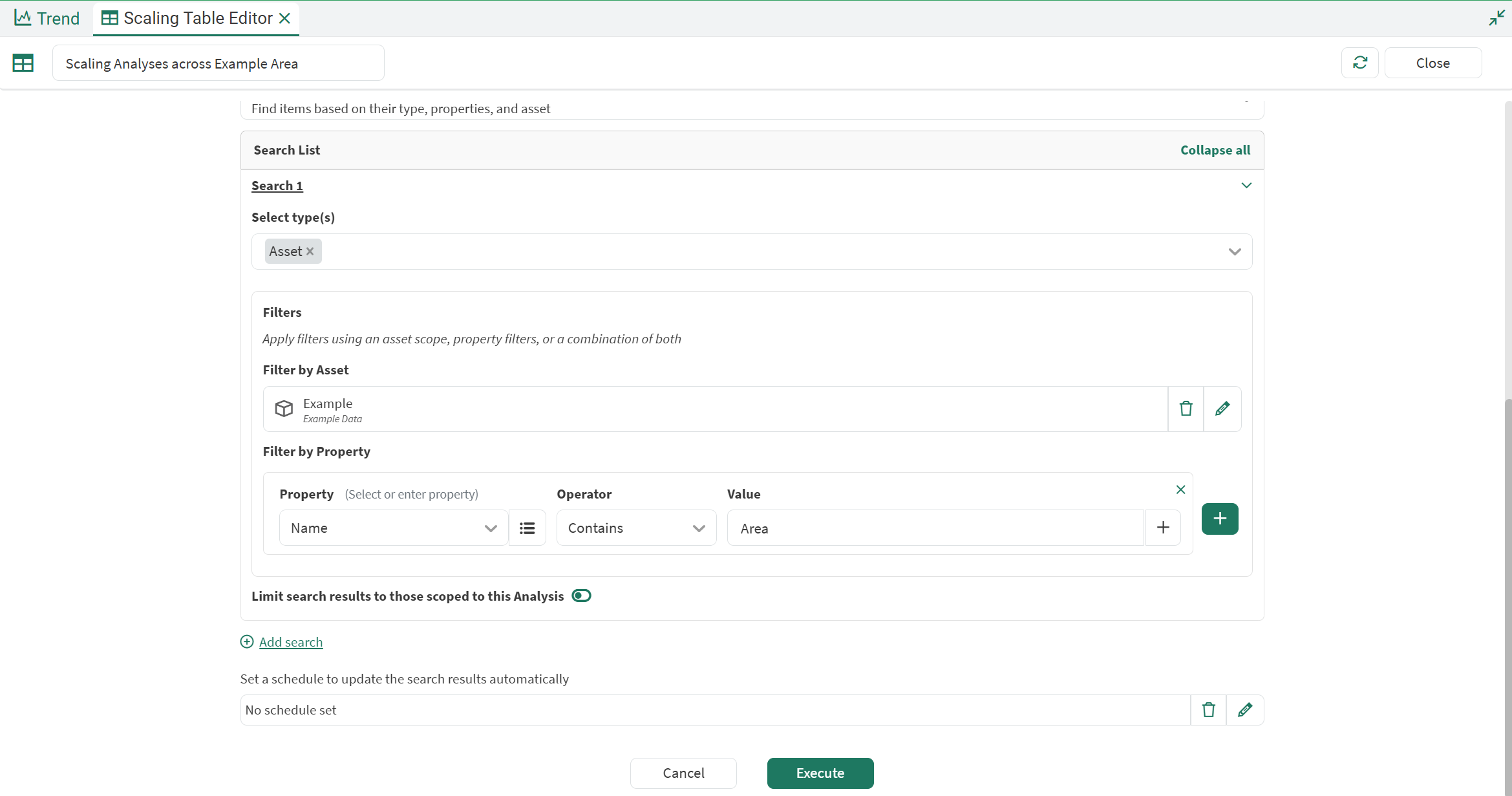
Because I am planning to perform a multi-variable analysis, leveraging multiple signals that are descendants of my target Assets, I begin by searching by using a Property Search with the following configuration:

• Type: Asset

• Filter by Name “contains” Area

• Further filtered by the parent node of my Example Asset Tree

Step 2: Review search results and find descendants I need

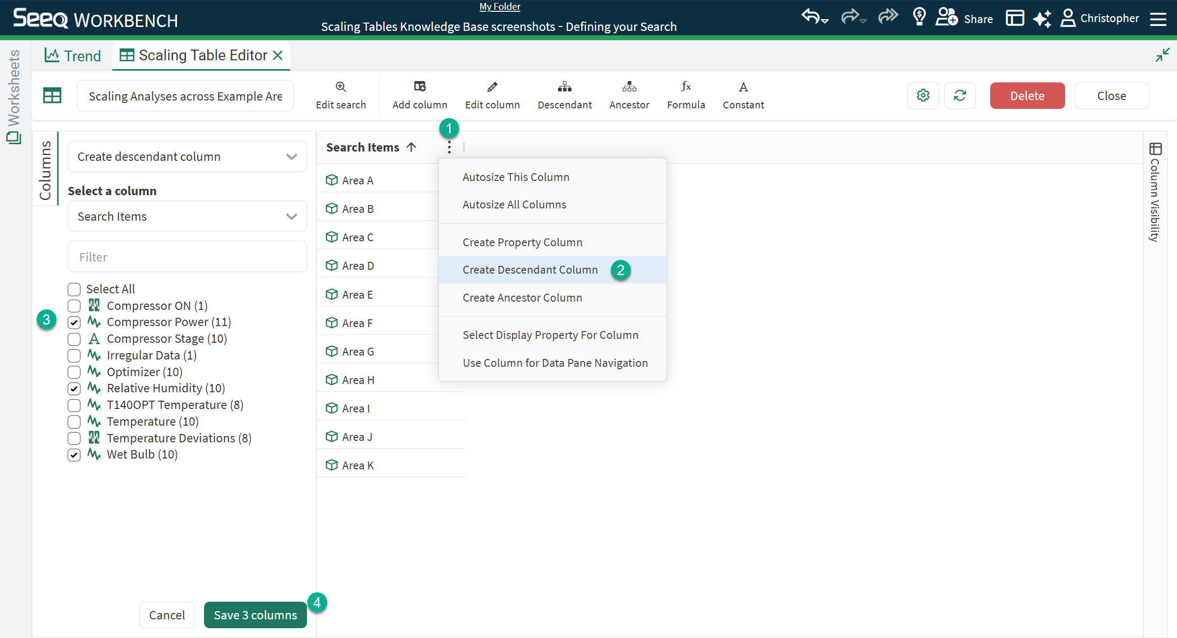
If you are happy with your search results, shown in the first, and single column “Search Items”, navigate to the three-dot menu in its' header, choose “Create Descendent Shortcut Column”, select the descendants that you want to include in your downstream calculations, and click Save.

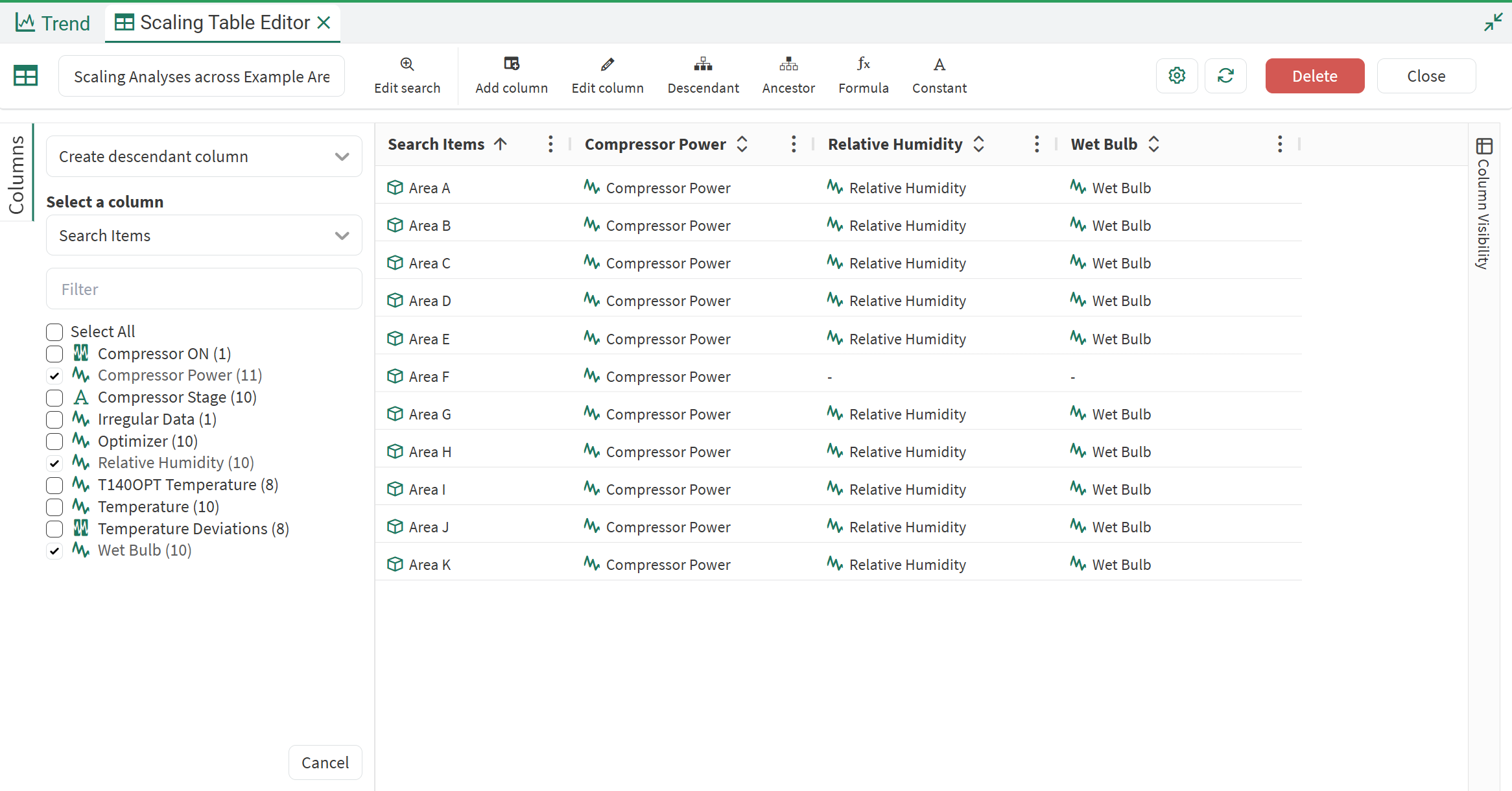
The results in your Scaling Table should look something like this:

Step 3: Configure your Formula

Now that your table has the inputs you need, you can select “Add Column” and the “Formula Creator” rule. Don’t forget to rename your column to something relevant to what you are doing.

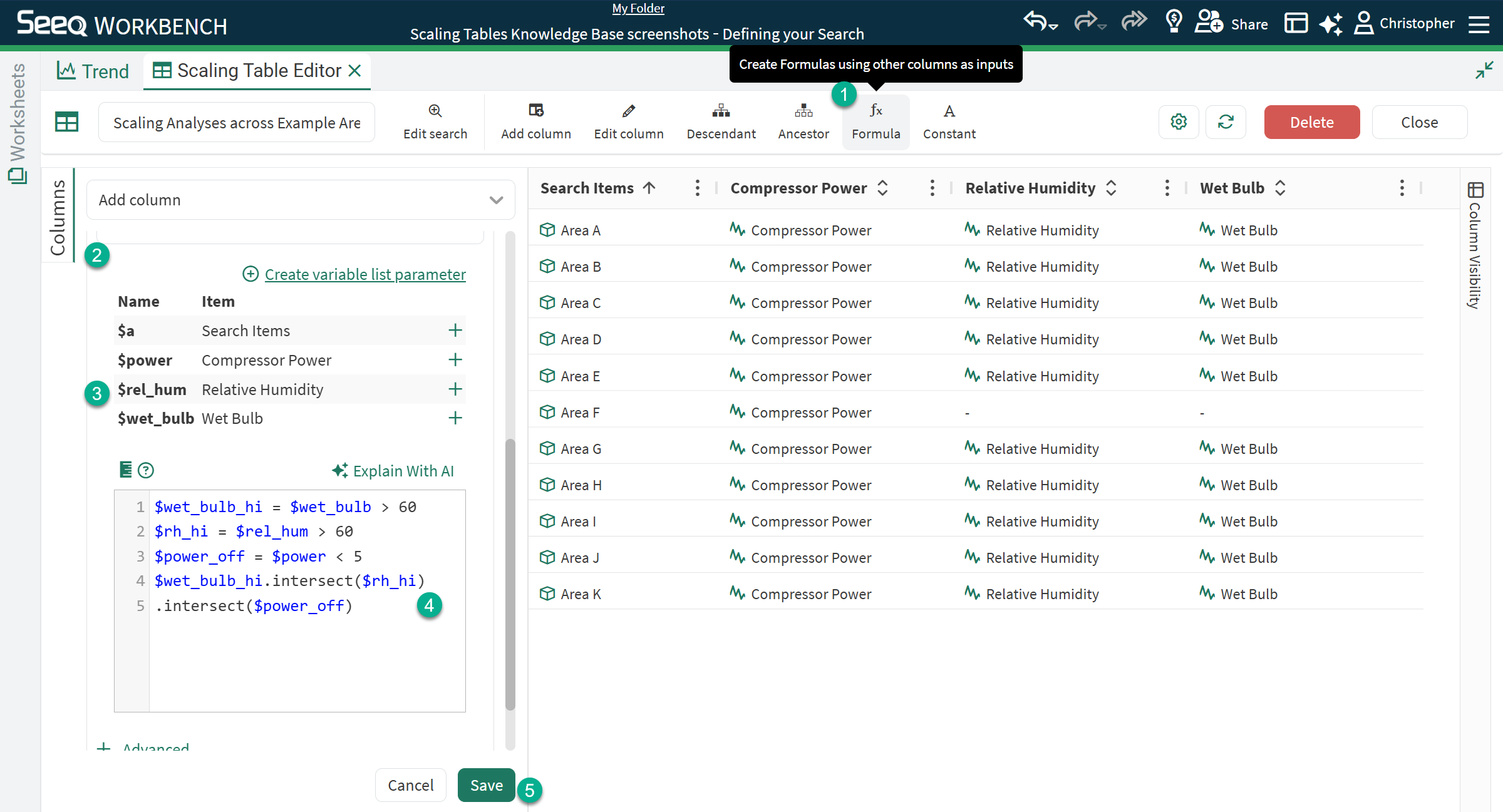
The “Formula Creator” rule allows you to the use the same Formula editor available in Workbench, but in Scaling Tables, configures a new column that will configure this calculation for every row that is successful. In the below example, I used a large, composite Formula of many sub-calculations, but you could just as easily created four separate Formula columns. The below Formula is being used to detect “Compressor Anomalies” - essentially I (as an SME) want to know when my compressors are not running but I have a high wet bulb and high humidity, which indicates to me we should be running the compressors.

$wet_bulb_hi = $wet_bulb > 60
$rh_hi = $rel_hum > 60
$power_off = $power < 5
$wet_bulb_hi.intersect($rh_hi)
.intersect($power_off)

Once you save your configuration, you’ll see a new column get created with an indicator of success or failure on your rule execution:

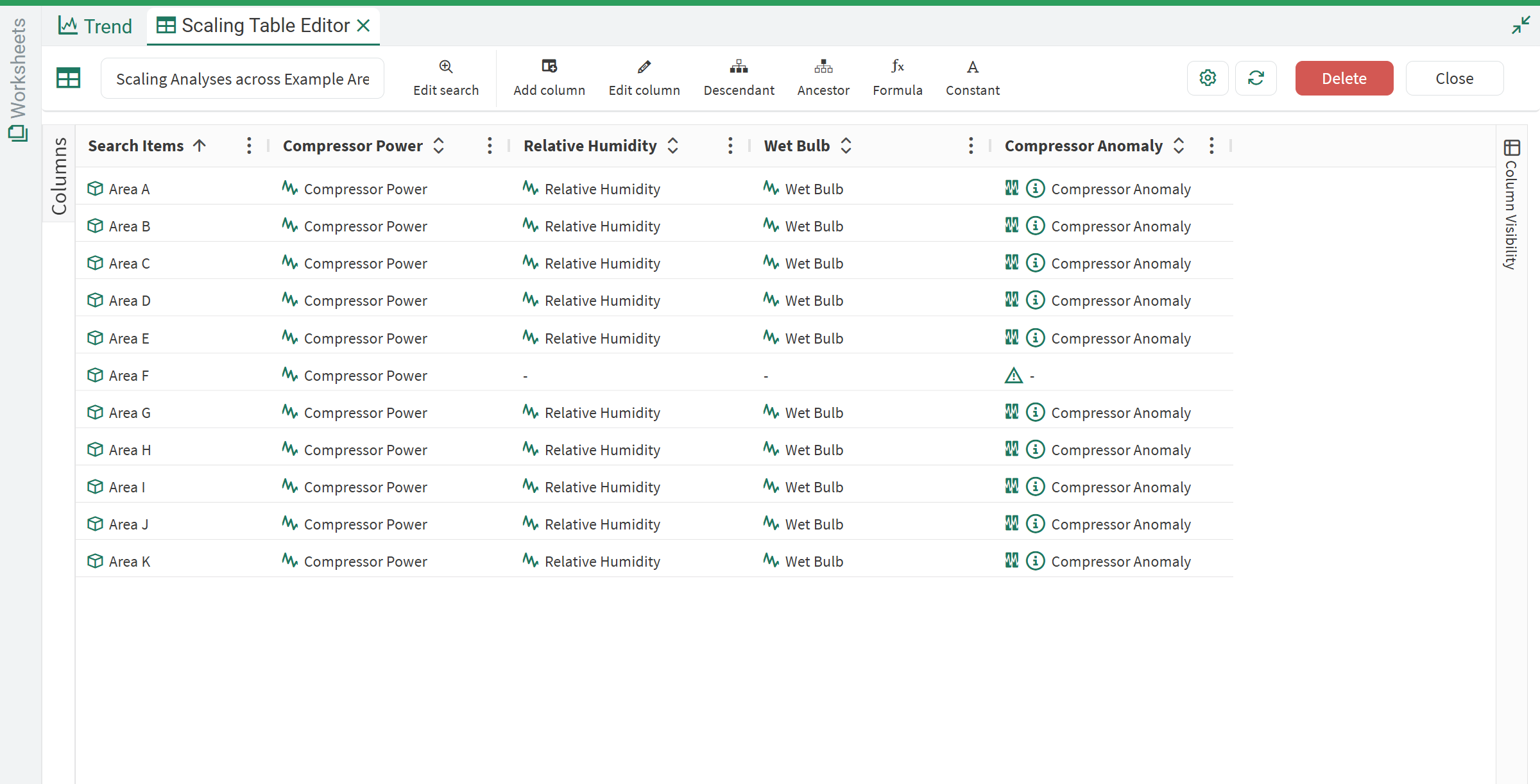
Note that Area F did not successfully calculate because we are missing Wet Bulb and Relative Humidity inputs. In the next step, we’ll address that.

Step 4: Add a fallback rule

To handle asymmetry in your fleet, you can add fallback rules to any column configuration. Here, we will perform a fallback Formula but the same flow can be applied for any column in your Scaling Table.

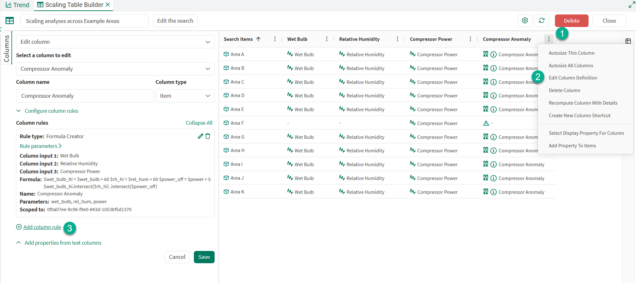
To edit the column we just created, click the three-dot menu in its' header and select “Edit column definition”, followed by “+Add column rule” underneath the first configured Formula:

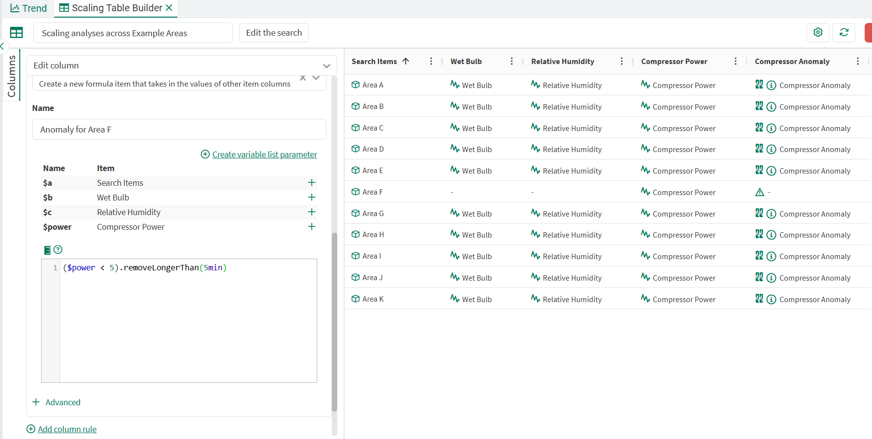
Then, create a new Formula that will be compatible with the descendants available for Area F, in this case only Compressor Power. For this compressor, we want to know if the machine shuts down (power < 5) for less than 5 minutes, indicating a short stoppage that can cause excess wear on the machine.

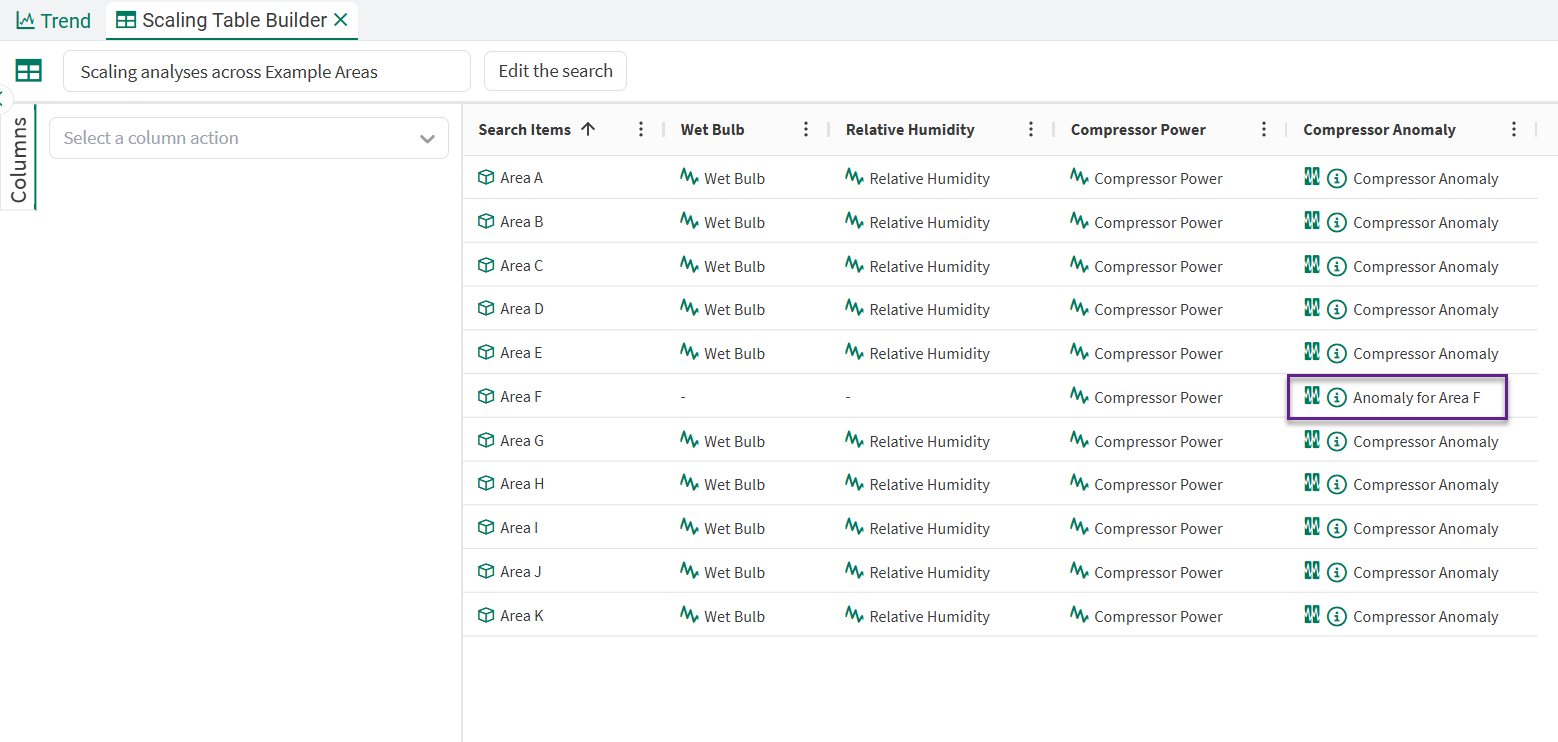
Once saved, we see the previously error state clear, and replaced with the new Condition:

Step 5: Trend and analyze the results

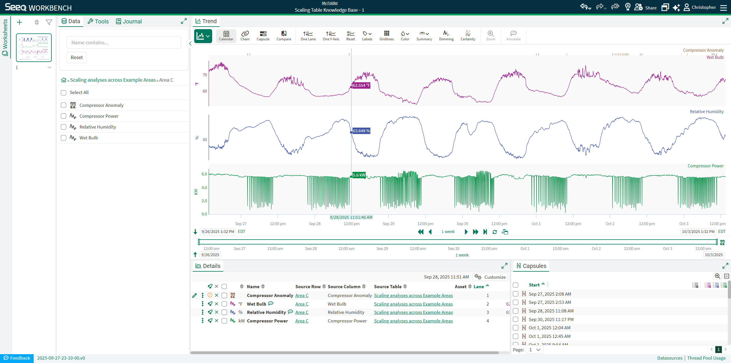
With our analytics configured at scale, we can navigate the table via the Data Pane now and add Area C’s results to the Trend.

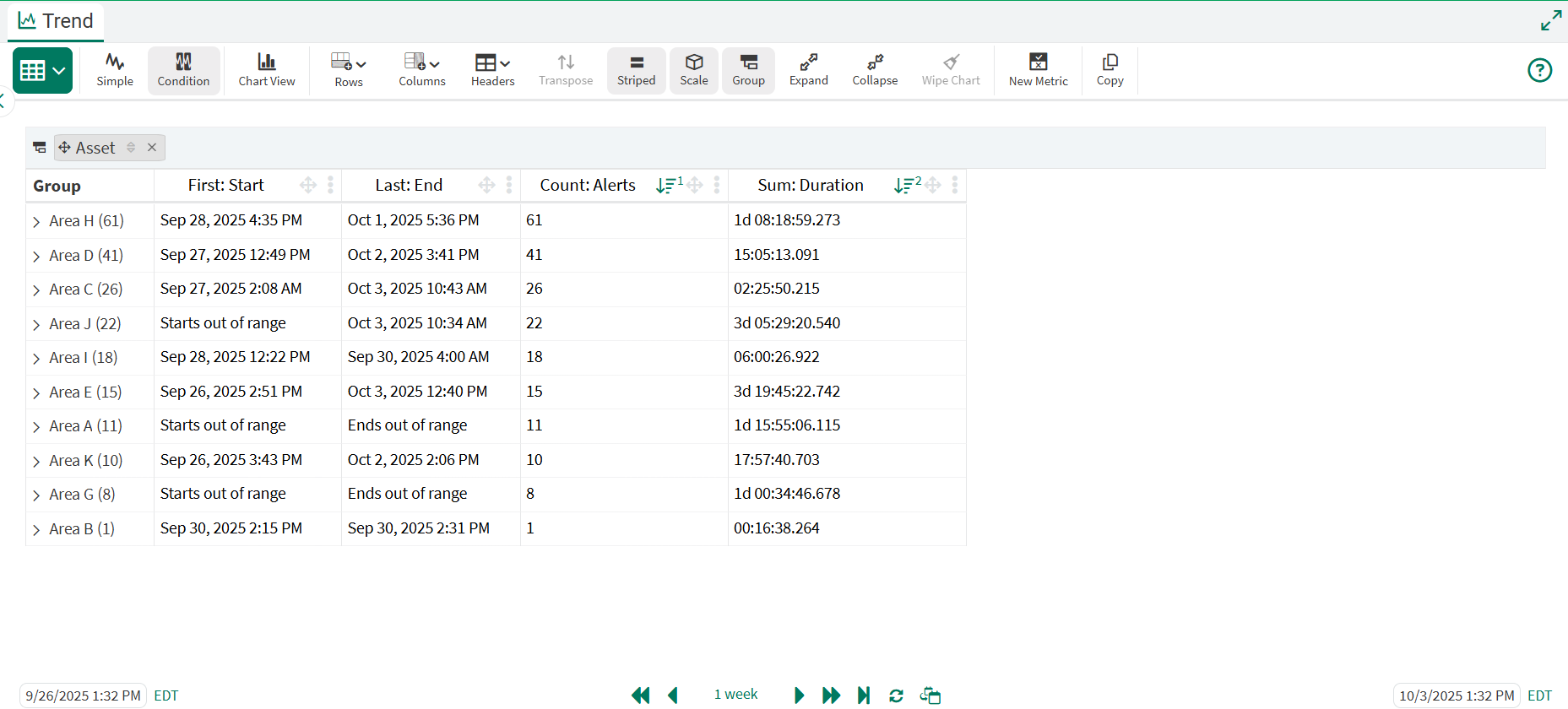
To get a view across all of our compressors, we can toggle the Trend type to Tables & Charts, then along the toolbar, select the Condition Table option and click the “Scale” icon.

After choosing the columns and headers I wanted for my view and grouping by Asset, I now have a table of all my capsules produced by the Conditions we configured in Scaling Tables to begin digging into my worst offenders.

This same methodology can be used to scale use cases to tens of thousands of assets, sending your conditions to monitor to Vantage as well as leveraging your favorite Workbench visuals as shown in this example.