Filtering to Remove Long-term Drift in Data

Overview

Process improvement workflows often involve identifying and quantifying relationships of interest between process variables. Long-term trends in data (such as slow drifts) can mask these process relationships, particularly when the magnitude of the long-term trends is significant relative to the modeling features of interest. High pass filtering can be used to remove these long-term data trends prior to analysis, resulting in much more accurate analytical results.

Characteristic Data Features to Consider

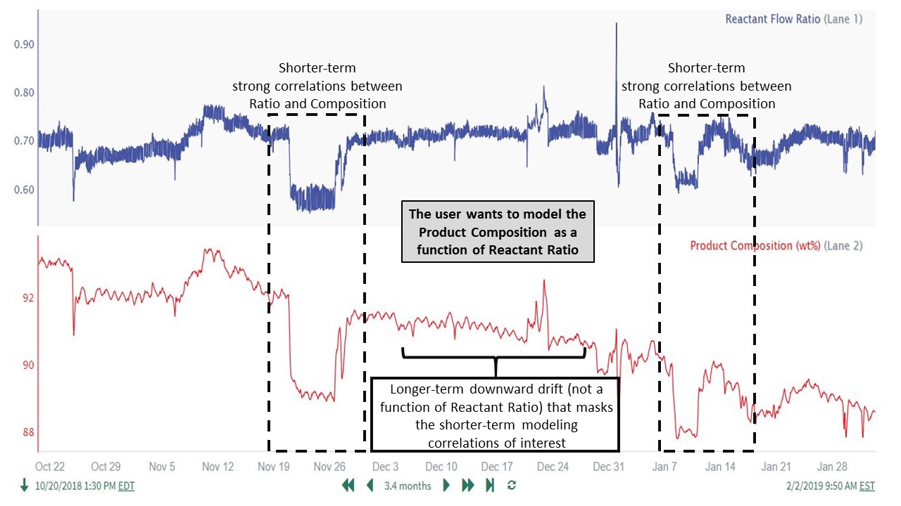
In a typical situation, the data contains significant longer-term features, but there is an important shorter-term relationship between multiple variables that the user wants to analyze and quantify. Simply doing a regression model on the raw data leads to a poor correlation or misleading results, due to the unrelated longer-term data features. As an example for prediction modeling:

The nature of industrial processes often produces these longer-term drift (or non-stationary) features in the data. It is important for the user to understand how these non-stationary data features affect the process relationships that are being modeled. Where the non-stationary features interfere with modeling objectives, appropriately selected high pass filtering can effectively remove them and greatly improve analytic results.

Stationary Time Series

A stationary time series is one whose properties such as mean and variance do not change over time (one with no predictable patterns in the long-term). Plots of stationary time series will be roughly horizontal. In contrast, many industrial time series signals are non-stationary due to seasonality, equipment fouling, instrumentation issues, etc.

A similar high pass filtering approach can also provide value for single process variables (analyzing a shorter-term feature) as well as other types of analyses (e.g. frequency analysis).

Common Industrial Applications

High pass filtering to remove long-term drift/features is a data pre-processing step that finds common use in many areas. Two examples are:

• Prediction modeling, to narrow the focus to shorter-term correlations of interest

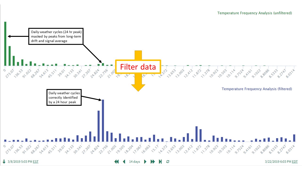
• Frequency analysis, to remove effects of 1) longer-term features and 2) the average signal value. In frequency analysis, both of these characteristics produce significant power peaks at very low frequencies, masking higher frequency power peaks that are often of more interest. For more information on these applications, please see (link to article to be developed).

Example benefits of using high pass filtering for these applications:

General Application Steps

The general procedure for applying a high pass filter is similar across most applications: remove the unwanted longer-term features while ensuring that the shorter-term features of interest are not significantly affected by the filtering.

A typical procedure for applying high pass filtering prior to prediction modeling is as follows:

1. Trend the data for the signals of interest. Determine the time window for prediction modeling.

2. Perform data cleansing to remove outliers, downtime periods, etc.

3. Based on a process understanding of the signal interrelationships, identify any longer-term data features that will interfere with the modeling objectives. These features could be present in the model's input signals and/or the "signal to model". At this point, also consider the potential need to align the signals if there are time lags or delays in the relationships.

4. Apply high pass filtering to each signal as needed to remove these longer-term features that would otherwise interfere with obtaining accurate modeling results. Use caution to ensure that features being removed are unrelated to the modeling relationships being identified.

5. Proceed with prediction modeling using the filtered data.

Guide to High Pass Filter Parameter Selection

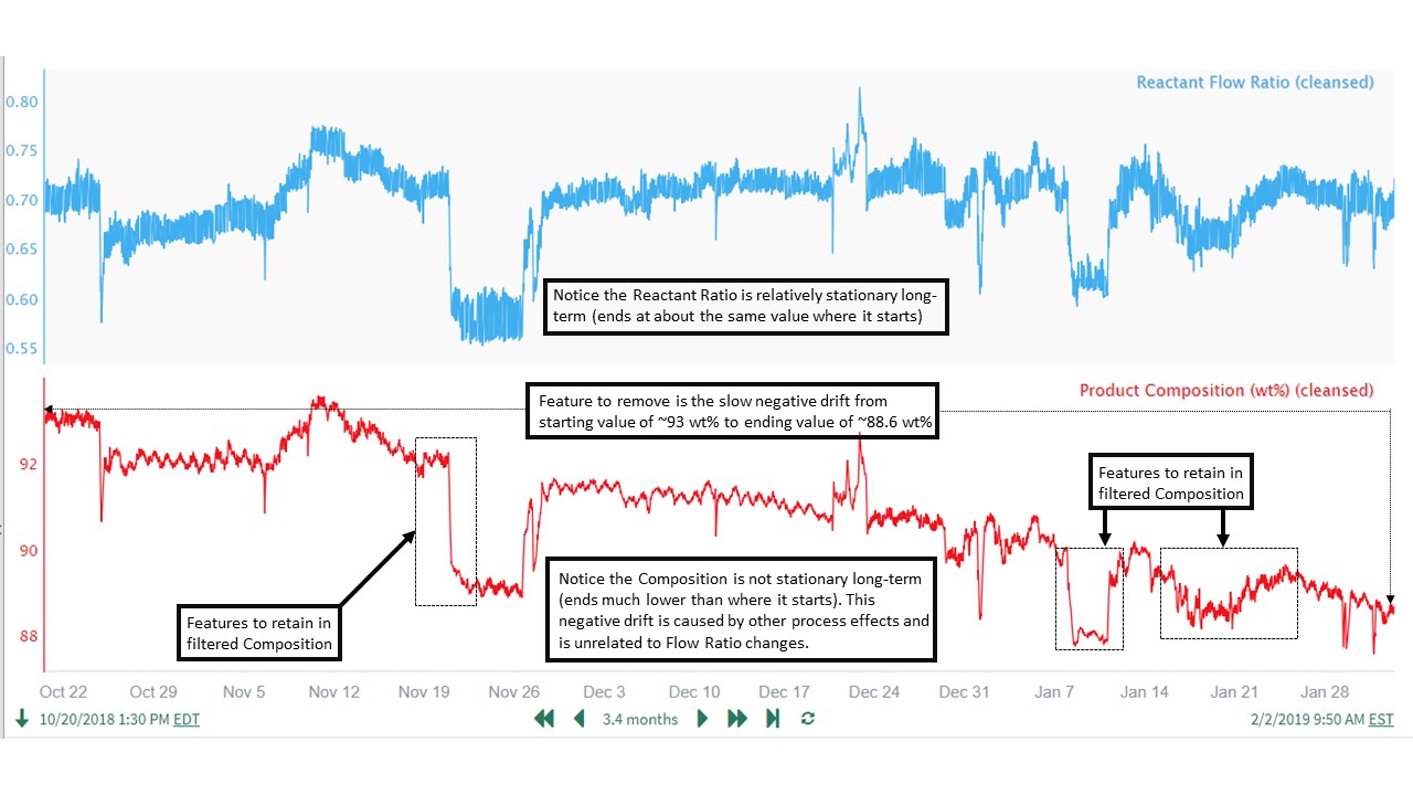
The parameter values selected for use in the high pass filter depend heavily on the data features that we want to retain and remove. To illustrate, we will use an example data set where our goal is to develop an accurate model between Reactant Flow Ratio and Product Composition. The features that we want to retain are the changes in the Product Composition due to changes in Reactant Flow Ratio. We need to remove the long-term drift feature in the Product Composition, as this variability in Composition is not caused by the Flow Ratio. As seen in the data, these Reactant Flow Ratio effects on Product Composition can happen over short time periods (less than 1 day) as well as much longer time periods (5-10 days). Fortunately for our filtering and modeling purposes, both ranges of time are very short relative to the long-term drift occurring over weeks and months. Therefore, a high pass filter should be able to separate the features we want to keep from those we want to remove (several examples shown in trend below):

Based on the data trends, we want to:

• Retain features that occur over time windows of up to 10 days (longest feature is roughly January 15 to January 25)

• Remove the slow, long-term drift in Product Composition that occurs over the ~3 months (~90 days) of data we are analyzing.

The high pass filter function (implemented in Seeq's Formula Tool) takes up to three parameters: 

$Signal.highPassFilter(cutoff, period, taps), where:

cutoff is typically determined by looking at the waveform and choosing a cutoff time period that is shorter than the duration of waveform features that you would like to filter (remove)

period is the sample period of data for the resulting signal and helps determine the "window" fed into the filtering algorithm

taps helps determine the "window" fed into the filtering algorithm (window = period * taps)

The period and taps inputs should be adjusted so that the "window" of time is large enough to encompass the feature in the waveform you want to pass through the filter. For example, if you select starting parameters and are not seeing the expected filtering of the longer-term features, then you likely need to increase the period and/or taps inputs to lengthen the time window.

The main input to select is the filter's cutoff (defined as frequency or period). Because time periods (that is, seconds/minutes/hours rather than Hertz) are easier to relate to the process data, we will work with the cutoff period (instead of cutoff frequency).

Working in Frequency or Period Units

Seeq allows using either frequency or period units. These are interchangeable, as the frequency and period are related by the equation: frequency = 1/(period in seconds).

A high pass filter removes features occurring slower than the user selected cutoff period. As a start we should pick a cutoff period much greater than 10 days (to retain our Reactant Ratio to Product Composition effects) and pick a value less than the time range over which the drift occurs. As a starting point, we choose an intermediate value of 50 days (1200 hrs) for the cutoff period, roughly halfway between our 10 day basis and the ~90 day length of data (though hard to quantify, we'll assume our drift feature time period is ~90 days).

We start with a high pass filter implemented with the formula listed below. We choose a 60 min period for 2 reasons:

• Our data features of interest occur over time periods of hours and days, so we need a long time window (period * taps) to achieve the desired filtering. Using a period much longer than our base data sample time will help achieve a long time window.

• We want the resulting filtered signal to have a sample period fast enough to include multiple data values in an 8-10 hour period, as some of the significant flow ratio changes occur within these time ranges. This requirement means we do not want the period to be higher than 60 minutes, as we will lose data granularity during important features (ratio changes resulting in composition changes).

We initially choose to leave the taps input (third parameter) at its default value of 33. (We plan to keep the period at 60 min and increase the taps later as needed to obtain the desired filtering characteristics.) Our starting high pass filter is then:

// High pass filter using a cutoff of 1200 hours. Choose 60 minutes as the period, use default for taps. Add a bias of 91 to recenter the filtered data around the normal operating range.
$Composition.highPassFilter(1200h, 60min) + 91

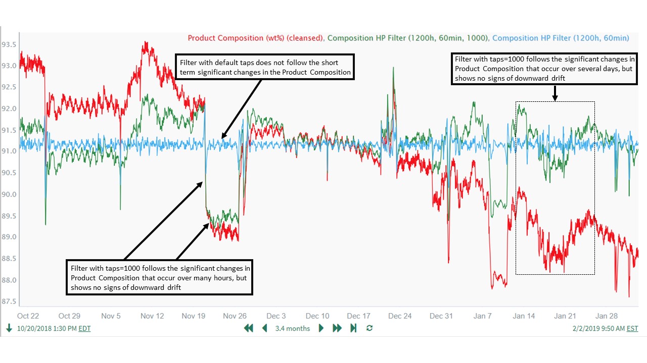
As shown in the trend below, this resulted in a poor performing filter ("Composition HP Filter (1200h, 60min)") which did not follow the short-term significant changes in Product Composition resulting from Reactant Flow Ratio changes. Increasing the number of taps makes the filter more selective about features retained and removed relative to the cutoff period, so the next logical step is to begin increasing the taps value. We then experimented with increasing the number of taps from 33, finally settling on a value of 1000 to achieve the desired filter characteristics. Needing a very high value for taps to achieve good filtering performance was expected, because the cutoff period is very high in relation to the chosen sample period of 60 min.

// High pass filter using a cutoff of 1200 hours. Choose 60 minutes as the period. Use taps = 1000 to achieve the filtering characteristics. Add a bias of 91 to recenter the filtered data around the normal operating range.
$Composition.highPassFilter(1200h, 60min, 1000) + 91

The formula above resulted in a filter ("Composition HP Filter (1200h, 60min, 1000)") which tracks the shorter-term Product Composition changes well, but remains stationary overall (in terms of having a relatively constant long-term mean) and does not drift downward over the course of the 3 month time period. Therefore, a high pass filter with these parameters achieves our goal for filtering the Product Composition signal:

Note that additional testing (not shown) using reduced filter cutoffs of 600 hours and 300 hours did not perform as well as the 1200 hour cutoff. This provided additional confidence in the final value used for the filter cutoff.

In summary, the filter cutoff should be chosen based on user insight and process understanding of the signal variability that is to be retained versus removed and on the approximate time ranges over which the variability occurs. The filter cutoff is the most important input, but the period and taps often need to be optimized (iterating from starting values) to get the desired filtering results. 

Impact of Period and Taps

For more detailed info on the impact of period and taps, refer to Steven Smith's book on digital signal processing. It's freely available by chapters on his website. The relevant chapter for this topic can be found here.

Example Application: Predicting Product Composition

In this example application, a Product Composition is highly correlated with an upstream Reactant Flow Ratio, and we wish to quantify this relationship with a linear regression model. Prediction modeling with the raw data gives poor results because there is a long-term downward drift in the Product Composition due to catalyst deactivation. High pass filtering greatly improves modeling results, as it allows us to isolate the effects of Reactant Flow Ratio on Product Composition.

Step 1: Inspect the Data Trends

The user trends the data over the desired time range and notices a strong correlation between the 2 signals, and therefore plans to model the Product Composition as a function of Reactant Flow Ratio. The user also notices a slow downward drift in the Product Composition data that does not correlate with Reactant Flow Ratio (see the first trend in Guide to High Pass Filter Parameter Selection above for more details on the data features):

Because the user plans to use a linear regression model to predict Product Composition based on Reactant Flow Ratio, the user also checks to see if there are any time delays or time lags in the relationship between the two variables. If there are, these will have to be compensated for with appropriate time shift (and possibly time lag) calculations, as the linear regression modeling tool does not handle dynamic relationships (it simply predicts the signal at a given timestamp as a function of the input signal(s) at the same timestamp). Zooming in on a large change in Product Composition to check for time delays and lags:

There is no evidence of dynamic relationships between the 2 signals, as they move together and are not offset relative to one another. Therefore, for this data, the user will not have to align the signals by compensating for time delays and lags.

Handling Dynamic Relationships in Prediction Modeling

Dynamic relationships are common in process data and must be handled appropriately when doing prediction modeling. (link to a separate article, to be developed) 

Step 2: Perform Data Cleansing

Before proceeding further with analysis, the user performs an intermediate data cleansing step to remove a high spike in the Reactant Flow Ratio. The user judges this to be the the only outlier data that needs to be removed:

// Remove high spike in reactant ratio (grow the bad data time period by 60 min to fully remove the spike)
$BadData = $Ratio.validValues().valueSearch(2day, isGreaterThan(0.85), 5min, isLessThanOrEqualTo(0.85),5min)
$Ratio.remove($BadData.grow(60min))

Note that we also use the same approach to remove the corresponding composition spike time period and generate a cleansed Product Composition signal. Both cleansed signals are used in the steps below.  

Step 3: Identify Data Features to Remove

A scatter plot of the cleansed Reactant Ratio and Product Composition implies there is a weak correlation between the two signals, though the user knows (from process understanding and data inspection) that there is a strong correlation:

The unrelated downward drift in the product composition can be clearly seen when plotted in the same lane with the cleansed Reactant Flow ratio:

Based on these observations, the user concludes that the longer-term downward drift in the Product Composition is significant and needs to be removed prior to prediction modeling. It is also important to note that only the Product Composition needs to be filtered in this example. (The Reactant Ratio does not display longer-term features that need to be removed.)

Step 4: Remove Drift in Product Composition Using a High Pass Filter

Being careful not to remove the shorter-term features in the Product Composition that are highly correlated with Reactant Ratio, the user adjusts the high pass filter settings to remove only the long-term downward drift in the Product Composition. The user chooses a cutoff time of 1200 hours because the drift feature in the data is very slow (see the Guide to High Pass Filter Parameter Selection for additional information):

// High pass filter using a cutoff of 1200 hours. Add a bias of 91 to recenter the filtered data around the normal operating range.
$Composition.highPassFilter(1200h, 60min, 1000) + 91

Note that the High pass Filtered Product Composition (using the above formula) nicely tracks the shorter-term changes due to Reactant Ratio impacts, but is much more stationary overall relative to the unfiltered Product Composition. The high pass filtered Product Composition result (ending value at far right of trend) ends up close to its starting value, because 1) we've removed the slow drift and 2) the Reactant Ratio ending value is close to its starting value:

The user is happy with this result and is confident that the high pass filtered Product Composition will be much more suitable for identifying an accurate prediction model.

Step 5: Prediction Modeling Using the High Pass Filtered Product Composition

Repeating the original scatter plot using the filtered product composition data results in the expected (and accurate) strong correlation: 

The corresponding linear, OLS prediction model gives an r^2 value of 0.83 and quantifies the relationship as 14.4 wt% (Product)/1 unit (Reactant Ratio):

The prediction model captures well the significant shorter-term features of interest in the Product Composition:

In this example, high pass filtering the data to focus the prediction modeling on the features of interest produces excellent results.