Filtering for Step Changes and Long-term Drift Detection in Process Data
Overview
Industrial data analytics often involves finding features of interest in data. While there are many types of features, two common examples are step changes and long-term drift. Low pass filtering can be used to find both step changes and long -erm drift in data. Finding step changes can help with process modeling, detection of process upsets, and general process troubleshooting. Finding long-term drift can help with detection of process upsets and abnormal operation, which may be leading indicators of equipment failure, degradation, and process safety issues. This article walks through a worked example using a low pass filter to identify different features in the signal.
Step Changes and Long-term Drift in Process Data
Industrial process data often contains step change and long-term drift features. These features can arise from a variety of sources, including planned operational target changes, unintended process upsets, equipment degradation, instrumentation faults, etc.
Examples of step change and long-term drift features are shown here:
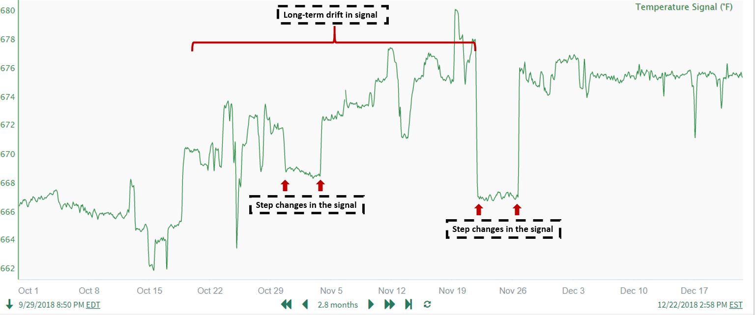
Analytical methods to detect these features can provide significant value in terms of process understanding, performing calculations, and detecting abnormal operation. The low pass filtering approach outlined in this article (and demonstrated with a detailed example application) can be used to detect step changes and long-term drift in data.
Data Smoothing
Depending on the nature of the process data and the analysis goals, we may select different types of filters for data smoothing. For the examples in this article, we will use a type of low pass filter, called Agile Filter due to these advantages:
varying amounts of signal smoothing are easily achieved with a simple input parameter selection
gaps or holes in the data are handled well (smoothing up to the edge of the gaps)
step changes are captured well while effectively removing systematic noise
Please see Intro to Signal Smoothing Filters for additional details around filter selection.
Guide to Agile Filter Parameter Selection
In this article we illustrate a type of low pass filter named Agile filter (see Intro to Signal Smoothing Filters for further information). Just as for other types of low pass filters, agile filters smooth the process data. The amount of smoothing is determined by the user selected input parameters. Agile filter passes low frequencies and blocks (or more accurately, significantly attenuates) high frequencies. This filter is particularly well suited for signals with discontinuities, as the output signal will be quite responsive in tracking to large jumps that hold steady afterwards. In addition, this filter is also well suited for signals with gaps or holes, as it smooths right up the edge of the gap.
In Seeq's Agile filter implementation via the Formula Tool, the user can specify 2 input parameters: period and window size. The period is the time period at which the input signal will be sampled, and the window size is the length of the process data that the filter can see during its computation. The window size defaults to 33 if not specified, resulting in a process data window size of 33 times the user selected period. The Agile filter can be applied very easily with this formula syntax:
$signal.agileFilter(1min, 33)By increasing the period or window Size parameters, we increase the amount of smoothing, removing more and more higher frequency variability while retaining lower frequency features.
In this example, a temperature signal is filtered with:
an Agile filter with a period of 1 min and window size equal to 33 (Agile_Filter_Basic)
an Afilter with a period of 4 min and window size equal to 33 times of the period (4*33) (Agile_Filter_changed)
an Agile filter with a period of 15 min and window size equal to 33 times of the period (15*33) (Agile_Filter_Very_Smooth)
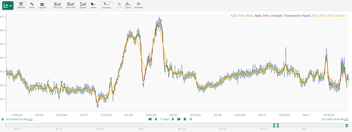
The effects of additional smoothing are obvious. The agile filter input parameters can be easily varied and fine tuned to generate the desired amount of filtering, based on the combination of analysis objectives and process understanding.
Example Application
In this example application, a process temperature contains a series of step changes as well as a period of significant long-term upward drift. We will use low pass filtering in combination with rate of change calculations to identify these features.
First we would like to capture step changes in the temperature signal by performing the following steps:
Smooth the signal to remove high frequency noise (if needed). This helps distinguish high rate of change (due to real step changes) from high rate of change due to noise.
Calculate the rate of change of the smoothed signal.
Define capsules to detect a high rate of temperature change (an indication of step changes).
Following identification of step changes, we would like to capture long-term upward drift in the temperature signal by performing the following steps:
Smooth the signal to follow long-term trends. This creates a signal basis for identifying long-term drift (by removing shorter term features).
Calculate the rate of change of the smoothed signal.
Define capsules to detect a high rate of temperature change in combination with an increasing rate of change (an indication of long-term drift).
Step 1: Smooth the Signal to Remove High Frequency Noise
In order to remove the high frequency features in the temperature, we select the Agile filter and gradually increase the sample period input parameter (trial and error). The sample period input is increased until the higher frequency spikes and variability have been removed, but the smoothed result still follows the large step changes. For additional information on filter and input parameter selection, please see Intro to Signal Smoothing Filters and Guide to Agile Filter Parameter Selection. In this case, we are able to achieve the smoothed signal characteristics using a sample period of 50 minutes while keeping the window size input at its default value:
$signal.agilefilter(50min)
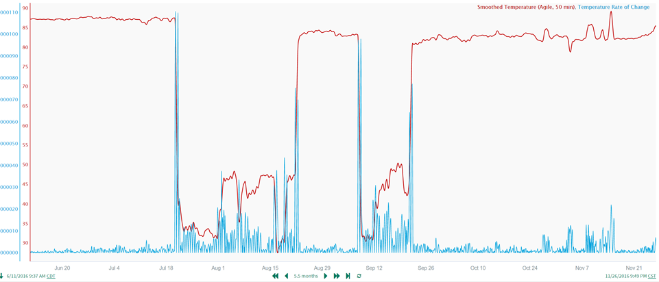
Application of the filter results in the following smoothed temperature signal:
Because the smoothed signal has removed the high frequency variability, the rate of change calculations in the next step can much more easily flag real step changes (and not falsely report high frequency features as step changes).
Step 2: Calculate the Rate of Change of the Smoothed Signal
We can now use Seeq's built-in formula functionality to calculate the rate of temperature change using the smoothed signal from Step 1. We do this using 3 functions:
RunningDelta() which calculates the temperature difference between the current sample and the previous sample
Derivative() of the RunningDelta() result, to determine how fast the temperature is rising or falling
Abs() to make it easier (in Step 3) to find positive or negative step changes
This is achieved with the following formula:
$signal_changes=$Smoothed_Signal.RunningDelta()
// By taking the absolute value of the derivative of the $signal_changes, we can capture the high amplitude changes in the signal which can be both in negative and positive direction.
$signal_changes.derivative().abs()
Application of the formula results in the following rate of change signal (based on the smoothed temperature signal):
We feel good about this rate of change signal because it has unique high values only during the step changes and therefore can be used with the Value Search tool in the next step to formally identify the step changes.
Note: while in this example we used a combination of RunningDelta() and Derivative(), the best approach for identifying step changes may differ somewhat based on the characteristics of your data. In some cases, using just the derivative() function may work well.
Step 3: Find Periods with Step Changes
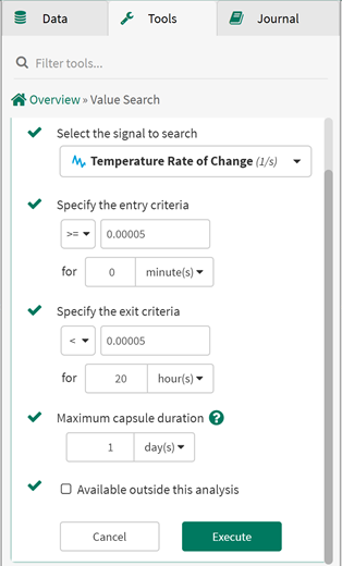
Next, using the Value Search Tool, we find the step change time periods by searching for where the temperature signal's rate of change is high (>0.00005). We also use an exit criteria time period of 20 hours, to prevent a large step change from possibly being flagged as multiple step changes. The Value Search input is shown below:
The results for the newly created Step_changes condition are shown below:
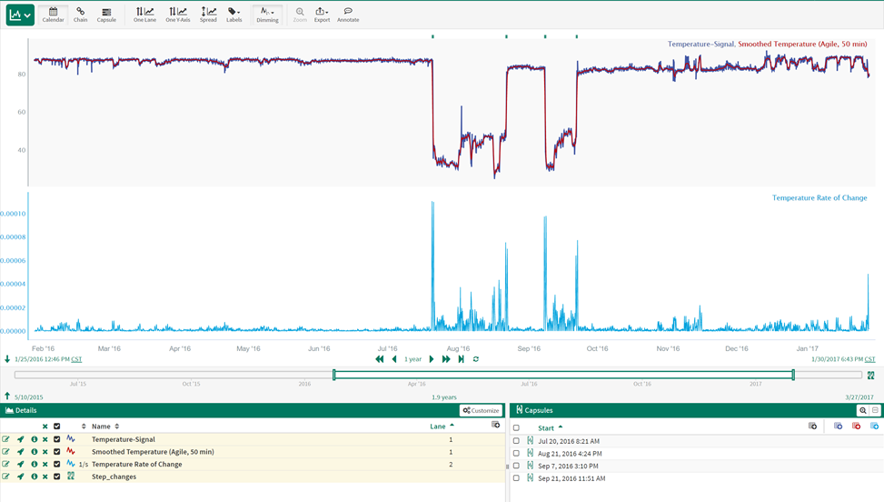
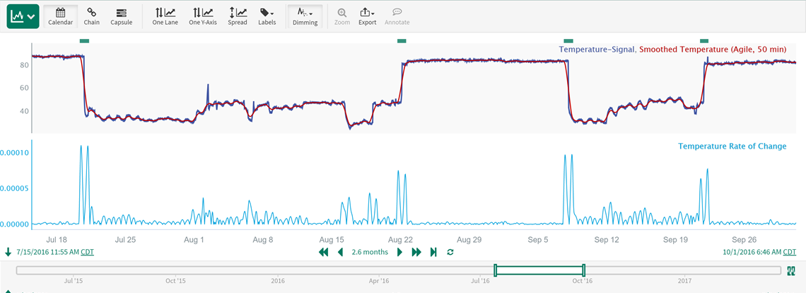
Zooming in we can see that the horizontal bars at the top of the screen (Step_changes condition) accurately capture the step changes in the temperature signal:
Now that we have these step change time periods captured, there are many additional analyses that could be done with them (for example, counting the number of step changes per day or week, calculating step change sizes, etc.), depending on our analytics goals.
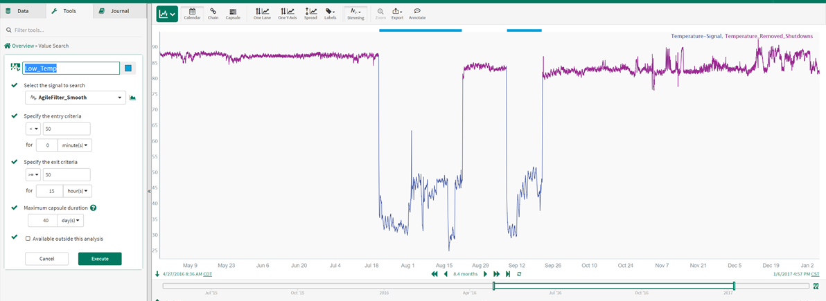
Note that in finding these step changes we have also included step change data where the process is in a shutdown state (where the temperature is less than 50 degrees Fahrenheit). If we only wanted to find step changes during normal operation, we would have first removed the shutdown data. As we move into the next step (finding long-term drift), we will remove the shutdown data before proceeding, as we are only interested in long-term drift when the process is running.
Step 4: Remove Shutdown Time Periods
We now begin the process of finding the long-term drift time periods in the temperature signal. Because these time periods are only meaningful when the process is running, our first step is to remove the shutdown time periods. To do this, we:
Use the Value Search Tool to find shutdown time periods, where the smoothed temperature from Step 1 is less than 50 degrees Fahrenheit. Then use the results of the Value Search to create the shutdown time periods (condition) and after that, use the formula to remove the shutdown data condition from the original temperature signal.
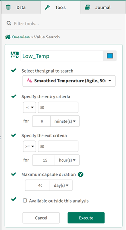
Use the Formula Tool to remove the shutdown time periods from the original, unfiltered temperature signal
// Grow (extend) the identified shutdown time periods to ensure the shutdown data is completely removed
$grow=$Low_Temp.grow(8 hour)
// Remove the shutdown data from the original temperature signal
$Temperature.remove($grow)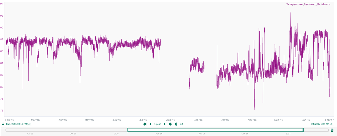
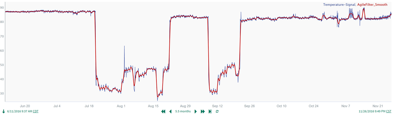
As a result, we have the Temperature_Removed_Shutdowns signal shown in the trend above, where there are data gaps during the shutdown time periods (as intended). We will use this cleansed signal in the next step. Note this is the original temperature signal without the smoothing applied in Step 1, as our smoothing filter created in the next step has a much different purpose.
Step 5: Smooth the Signal to Follow Long-term Trends
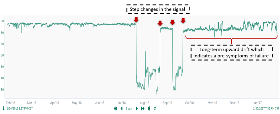
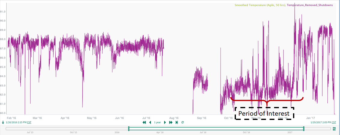
When we look closely at the long-term trend of the shutdown-removed temperature signal from Step 4, we see that before the first shutdown the long-term average temperature is relatively constant. During the last production run on the right hand side of the trend, the long-term average temperature started increasing slowly, particularly after September 2016. (While this long-term upward drift is difficult to detect in the unfiltered temperature signal here, it will stand out much more distinctly after we apply long-term smoothing.) These gradual, long-term increases in the temperature (see Period of Interest) are known to lead to process upsets and equipment failures if they are not detected quickly and addressed:
Therefore, it is valuable to use Seeq's analytics tools to automatically detect these gradual, long-term drift features in the data. First, we need a signal which captures the long-term trends in the temperature signal. To do this we will use the Agile filter function (used also in Step 1), but this time our goal is to remove high frequency as well as intermediate frequencies, so that we retain only the long-term behavior of the temperature. Whereas in Step 1 we used a "short-windowed" Agile filter (smaller amount of smoothing), here we will use a "long-windowed" Agile filter (to do a large amount of smoothing).
In order to remove everything but the long-term features in the temperature, we select the Agile filter and gradually increase the sample period input parameter (trial and error). The sample period input is increased until we see a filtered result that 1) represents the long-term characteristics of the temperature signal and 2) shows a smooth, distinct upward trend during the period of interest that we know we need to detect. For additional information on filter and input parameter selection, please see Intro to Signal Smoothing Filters and Guide to Agile Filter Parameter Selection. In this case, we are able to achieve the smoothed signal characteristics that we need (using a sample period of 50 hours) while keeping the window size input at its default value:
The formula (where signal is Temperature_Removed_Shutdowns) is:
$signal.agileFilter(50 hour)Application of this Agile filter gives the following filtered result:
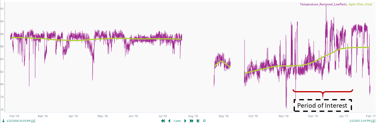
As you can see in the trend above, the filtered temperature tracks the long-term trends in the temperature well. The slow increase in the signal during the "Period of Interest" (which is difficult to visualize from the original data) is easily seen when looking at the filtered temperature.
Step 6: Calculate the Rate of Change of the Smoothed Signal
We can now use Seeq's built-in formula functionality to calculate the rate of long-term temperature change using the smoothed signal from Step 5. We do this using 2 functions:
RunningDelta() which calculates the temperature difference between the current sample and the previous sample
Derivative() of the RunningDelta() result, to determine how fast the temperature is rising or falling
This is achieved with the following formulas to generate two new signals named RunningDelta_AgileFilter (lane 2 in the trend below) and Derivative of RunningDelta (lane 3 in the trend below):
// RunningDelta of the Smooth_Temperature signal. The name of the resulting signal would be Delta_Temperature.
$Temperature_Smooth.runningdelta()// Derivative of RunningDelta
$Delta_Temperature.derivative()For trend visualizations, a zero signal is also created using this formula:
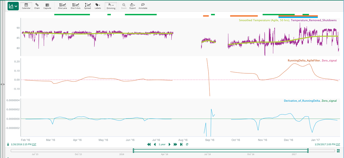
0.tosignal()Application of these formulas generates the new rate of change signals, which are plotted with the created zero signals to aid positive/negative value visualization:
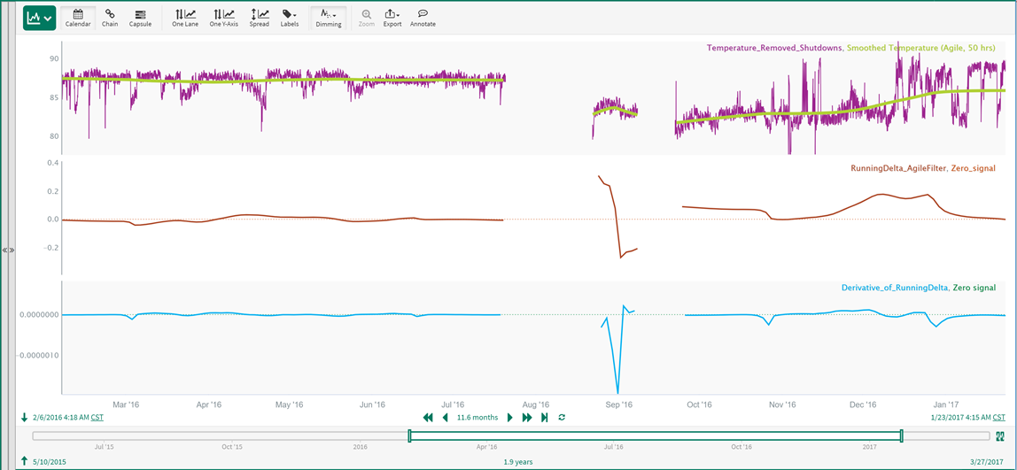
Zooming in, during the upward drift in the temperature that we want to detect, the RunningDelta_AgileFilter signal is well above zero and the Derivative of RunningDelta is also above zero:
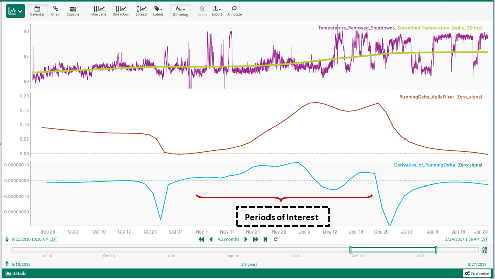
Based on this data, these characteristics are unique to the upward drift that we want to detect, so we can use these findings in the next step to develop an automated detection method.
Step 7: Find Periods with Long-term Drift
Now that we have rate of change signals based on the temperature signal smoothed to follow long-term drift, we need to use these signals to automatically detect upward drift events (such as the Period of Interest noted above).
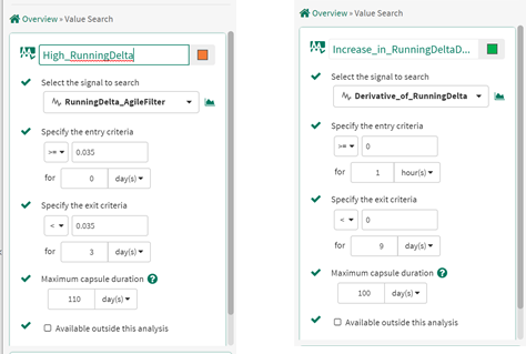
Based on the findings in Step 6, we use the following method to reliably detect the long-term upward drift "Period of Interest", without generating false drift detection. This method finds time periods where the running delta is positive (>0.035) and increasing:
Use the Value Search Tool to find periods where the RunningDelta signal is > 0.035, indicating the temperature is rising significantly (high running delta).
Use the Value Search Tool to find periods where the derivative of the RunningDelta is >= 0 (increasing running delta).
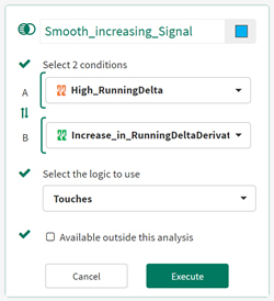
Use the Composite Condition Tool to combine the two time periods such that the result includes any time periods of high running delta, where those time periods touch increasing running delta periods.
To implement this method, we use the following inputs to the Value Search Tool to create new conditions for High_RunningDelta and Increasing_RunningDelta:
The new conditions are shown below, where the orange bars represent the High_RunningDelta condition and the green bars represent the Increasing_RunningDelta condition (where Derivative_of_RunningDelta is > 0):
Finally, we use the Composite Condition Tool to combine the 2 conditions. For the logic we specify when the High_RunningDelta Touches the Increasing_RunningDelta condition:
The Composite Condition gives this result where the "Period of Interest" (upward drift) has been successfully identified with our series of filtering and rate of change calculations:
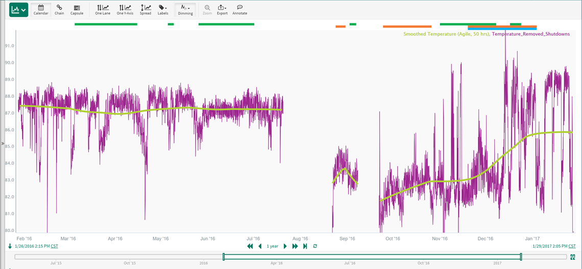
The new condition (Smooth_increasing_Signal, shown by the blue horizontal bar) detects the long-term, upward drift of concern to the process operation. Now that we have a method to monitor the temperature data for long-term increases, these Seeq calculations can be used going forward to warn the operations team of long-term upward drift events before they result in process failures or significant economic loss.
Note that in this example we were focused on long-term, positive (or upward) drift, because that was the feature of concern with this process operation. In other cases, it would be easy to vary the approach to find long-term drift in either direction.