Intro to Signal Smoothing Filters
Overview
Many analyses require signal smoothing in order to remove noise or certain data features. Seeq has various tools for smoothing signals. Each tool has its pros and cons; in this document we aim to help you understand what each filter is doing and when to use each one.
When to Filter
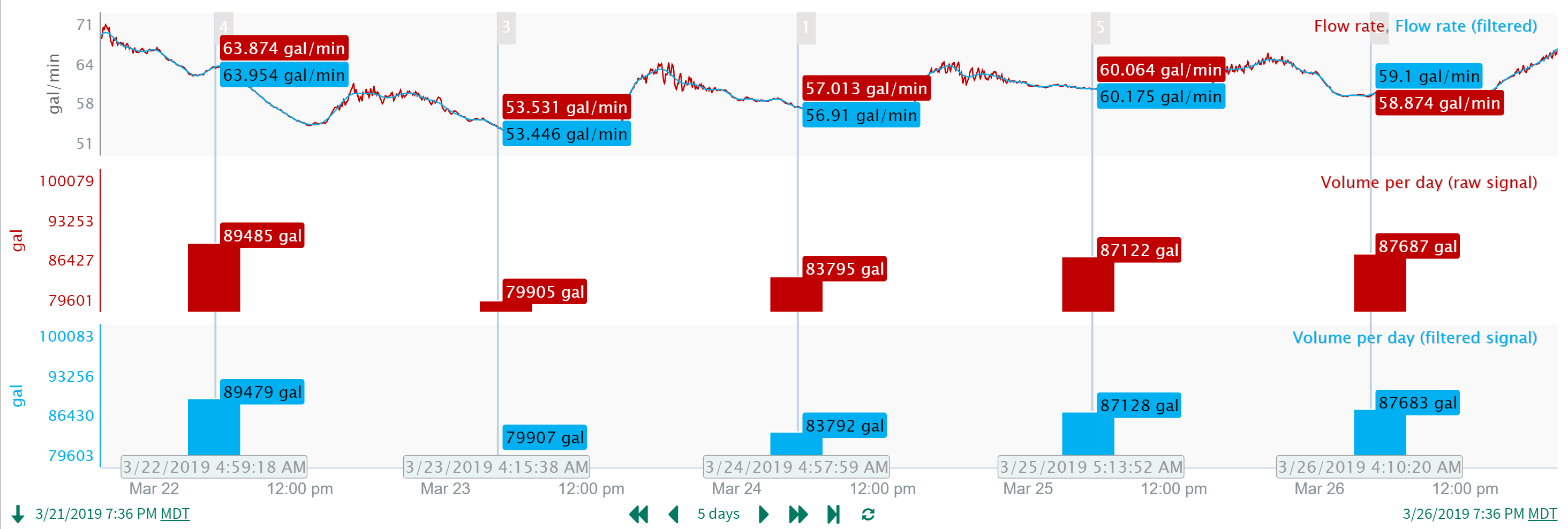
Filtering is computationally expensive and therefore takes considerable time and resources on server. Before using a filter in your analysis, consider whether one is required. In general, if you are doing an analysis that aggregates data over long periods of time you are unlikely to need a low pass filter (filters that remove noise). For example, if you are totalizing or averaging over a day and the noise in the signal is at a much higher frequency, there's really no need to filter since the noise will be effectively filtered out over the long duration summation. See the example below. Notice that the difference between the totalized volume calculated from the raw signal vs the filtered signal is very small compared to the total (only about 0.007%). Note: Under certain conditions a high pass filter can be useful in these situations.
Filter Definitions
Filters are classified based on their "frequency response". Things that happen very quickly are comprised of high frequencies. For example, spikes in a signal that last only a hand full of samples, or step changes in the signal value are high frequency features. Conversely, things that happen slowly are comprised of low frequencies. Seasonal drift or changes due to equipment degradation (e.g., clogging of a particulate filter) are examples of low frequency features. The exact definition of "high" and "low" is relative to how quickly the process you are monitoring changes. A common signal processing task is removal of "noise", which is frequently at a frequency greater than that of the process. For this reason, the most common filter in process analysis is the "low pass" filter which allows low frequencies through (the filter "passes" them) and blocks high frequency content. This has the effect of removing spikes, smoothing rapid transitions, and removing most kinds of noise.
The second most common is the "high pass" filter which allows high frequencies to pass, but blocks the low frequency content. This has two major effects: 1) it shifts the signal to have an average value of zero (since the lowest frequency in the signal is its overall average, the so-called DC offset), and 2) it removes slow drift which can happen over long periods of time.
Seeq has several low pass filters and one high pass filter. Some filters base their calculations on the samples in a fixed time interval on either side of the current sample, in the descriptions below, we call this the fitting window length. This is different than the number of input samples, which is used by the low pass filter, in which the actual number of data points is evaluated. The difference is subtle but important. The fitting window length can be specified for irregularly sample signals - the algorithm simply gathers all the samples within the specified time span. In contrast, filters that use number of input samples assume that the signal is regularly sampled, otherwise (in the extreme case) the algorithm might have to look infinitely into the past to find all the samples it needs. Therefore, before the low pass filter can be used on irregularly sampled signals, they must be resampled to a uniform sampling. This is done internally by the filter, but does have some usage ramifications, explained in the low pass section below.
Low Pass Filters
Agile Filter
The Agile filter can be used via Formula with the basic format of $a.agileFilter([output sample rate][fitting window length]). It uses the Loess method, also known as Lowess, local polynomial regression, or moving regression, which takes a window of samples and fits a line through them. It then uses the value of the best-fit line at the sample time to determine the filtered value. The 'agile' name is due to its particular ability to retain discontinuities (like step changes) while removing jitter and spikes. The output signal will be quite responsive in tracking large jumps that hold steady afterwards. In addition, this filter is also well suited for signals with gaps or holes, as it smooths right up the edge of the gap.
In signal processing terms, the agile filter is a non-linear filter and as such the exact frequency response cannot be determined ahead of time. Therefore, if you are trying to remove a specific frequency, you may not get the control you are looking for with this filter.
SG
The SG filter can be used in Formula with the basic format $a.sgFilter([fitting window length]). It uses the Savitzky-Golay method, also known as least-squares or DISPO (Digital Smoothing Polynomial), which works by fitting a polynomial (default of second order, but this can be specified) to a window of input data and deriving the output sample from the polynomial. Since the SG filter minimizes the least-squared error of the selected polynomial at each point, it has the ability to retain many high-frequency characteristics while removing erroneous data that cannot be be reasonably approximated using a locally fit polynomial. This filter is particularly suitable for signals with gaps or holes, as it smooths right up the edge of the gap.
Low Pass Filter
The Low Pass filter can be used in Formula with the basic format of $a.lowPassFilter([cutoff frequency], [output sample period], [number of input samples]). The Low Pass filter is a digital sinc filter which is fast and can provide precise frequency cutoffs. For example, if you know that your signal is contaminated with noise at 100 Hz, but what you are interested in is occurring at 90 Hz, you can design a low pass filter that has a cutoff of 95 Hz with very good blocking above that and very good passing below that. Importantly, as mentioned above, the low pass filter requires a uniform sampling period for the signal. To ensure this, the input is resampled to the output sample period before the input samples are collected and used for analysis. Therefore, to maintain the same time window, you have to increase number of input samples as you decrease the output sample period.
The Low Pass filter isn't as good as the Agile or SG filter at capturing discontinuities like steps, and also requires the full window of input samples to work. The latter point means that it won't filter up to the edge of signals, which can be a disadvantage for real-time monitoring.
Moving Average
The Moving Average filter can be used in Formula with the basic format of $a.aggregate(average(), periods([averaging duration], [output sample interval]), middleKey()). Technically, it's a subset of the SG filter family using a polynomial of order zero. It works by averaging the data in a given time frame and applying the average to a given sample. Moving averages are fast and good for removing truly random noise while retaining step features. For this reason they are common in digital signal processing where you see lots of steps (binary transitions from 0-1). Because noise is rarely truly random and they tend to let a lot of high frequency content through, they are poorly suited to signal smoothing.
High Pass Filters
Seeq implements one high pass filter which can be used in Formula by $a.highPassFilter([cutoff frequency], [output sample period], [number of input samples]). It's implementation is similar to that of the Low Pass Filter (i.e., it's a digital sinc filter), and for this reason, it has the same advantages and disadvantages as the Low Pass Filter.
Filter Demonstrations
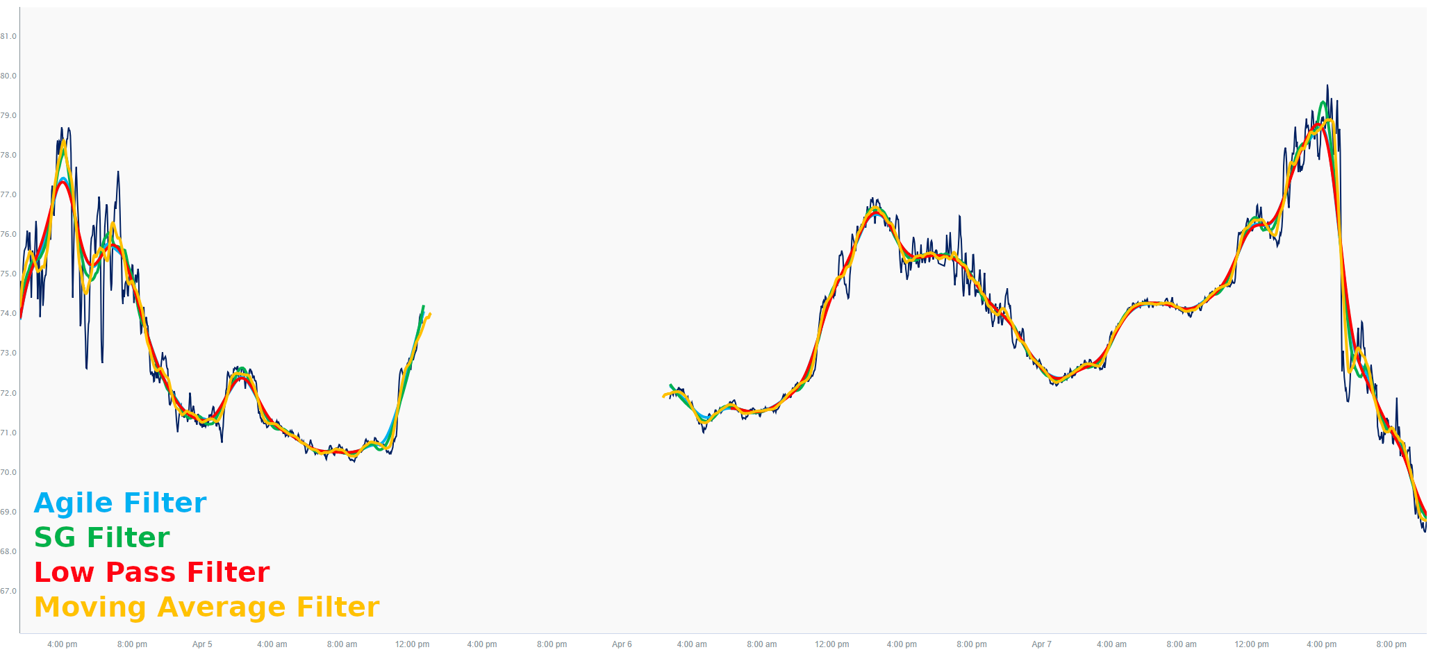
The image and table below compare the four smoothing filters. The filter data windows and other options (like cutoff in the case of the Low Pass filter) were selected to give similar performance in terms of data smoothing but also highlight their differences.
| Filter | Formula | Filter Data Window |
|---|---|---|
| Agile Filter | $a.agileFilter(5min) | 2.75 hrs |
| SG Filter | $a.sgFilter(5min) | 2.75 hrs |
| Low Pass Filter | $a.lowPassFilter(3hr, 125s, 200) | 6.94 hrs |
| Moving Average Filter | $a.aggregate(average(), periods(50min, 2min), middleKey()) | 50 min |
Getting Close to Edges
Depending on your application, the performance of the filter near the edges of your data may be critical to your filter selection. In the above image you can see that the that the low pass filter is not a good choice for real-time filtering or filtering around holes in your data. The output terminates at 1/2 * Filter Data Window away from the edge of the signal—nearly 3.5 hrs of unavailable data in this case! Conversely, we see that the moving average filter actually goes past the edge of the data by half its data window and would go even further if we used endKey() instead of middleKey() for the time of the output sample. Agile and SG terminate at the last sample, making them a good compromise of all the filters.
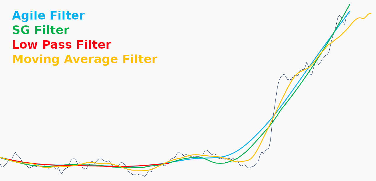
Step Changes
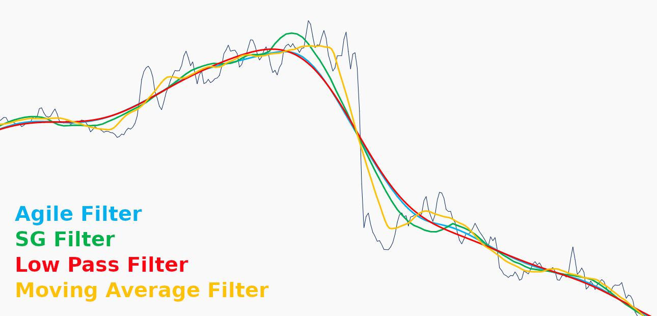
In the above image you can see how the filters respond to a step change in the data, this one taken from the right side of the first plot. The step is tracked best by the Moving Average, followed by the SG Filter, then the Agile Filter, and finally worst by the Low Pass filter. The SG and Agile Filters are compromises in this case.
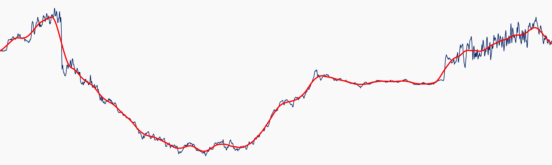
Noise Reduction
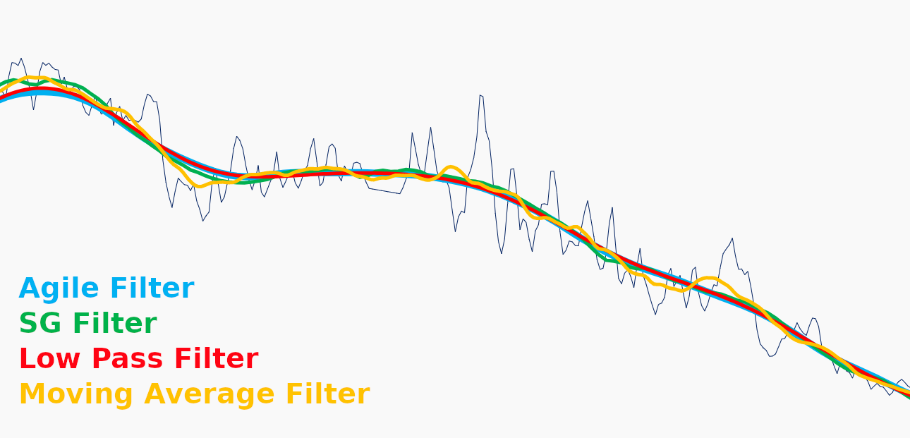
In this figure you can see the noise rejection of the filters. A close inspection reveals that the Moving Average does a poor job of rejecting this noise, followed by the SG filter, with the Low Pass and Agile preforming similarly. Notice that this is opposite of the step response: filters that perform well in tracking a step response will almost invariably do worse at high frequency noise rejection. However, for general smoothing applications, it is this inconsistent rejection of high-frequency noise that makes the moving average filter a poor choice for signal smoothing. Any of the other filters would be a more appropriate selection for this kind of task.
Output Shape
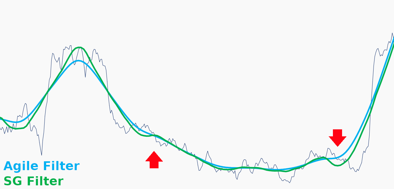
If you inspect the Agile and SG filters in the zoom box, you will notice how the shapes of the outputs relate directly to the fitting curves used in the filter. The Agile filter uses a linear fit and reacts slowly for a given window to oscillations, while the SG filter's quadratic fit (Seeq's default for the filter) allows it to track the curve more closely. The order of the quadratic used as the SG filter's basis function is settable in the equation and can be selected based on the requirements of your data. Higher order equations track the original signal better, exhibiting less noise rejection but better tracking of step changes.
Summary
| Filter | Pros | Cons |
|---|---|---|
| Agile |
|
|
| SG |
|
|
| Low Pass/High Pass |
|
|
| Moving Average |
|
|