Frequency Analysis
Fourier Analysis is used to convert a time series signal from the time domain to the frequency domain. Fast Fourier Transform (FFT) is a computational method used to perform Fourier Analysis on a discrete signal. The Frequency Analysis tool in Seeq leverages FFT to identify peak frequencies/periods in an input signal.
Using the Frequency Analysis Tool
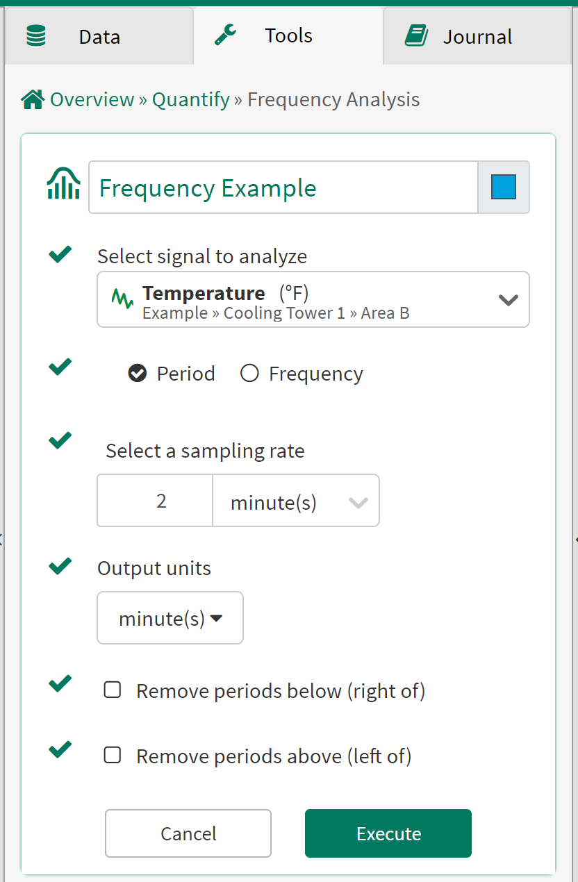
Signal to Analyze: From the dropdown menu select a signal from the details pane, pinned items or recently accessed sections.
Period or Frequency: Select Period to display the calculated FFT in units of time, or select Frequency to view the calculated FFT in units of frequency (for example, 1 Hz = 1/s). Note: Time-series data is typically not sampled at a rate faster than 1 second, so the option to view the results as periods is provided.
Sampling Rate: Enter the sample rate of your data. Based on the signal selected, this input is automatically generated but may be manually adjusted.
Output Units: From the dropdown menu, select the desired Period or Frequency output units of the FFT analysis.
Remove Periods Below (Right of): Check this box to truncate the FFT analysis output to the right of a specified value. If Period is selected above, this option truncates the results below the specified period. If Frequency is selected above, this option truncates the results above a specified frequency.
Remove Periods Above (Left of): Check this box to truncate the FFT analysis to output to the left of a specified value. If Period is selected above, this will truncate the results above the specified period. If Frequency is selected above, this option truncates the results below a specified frequency.
Available outside this analysis: Check this box to allow the calculated FFT to be used in other workbench analyses and topics. Checking this box makes the FFT available for all Seeq users and displays the FFT in search results. Selecting this option checks to ensure that the FFT has a unique name as the name is published to the global name space.
Sine Wave Examples
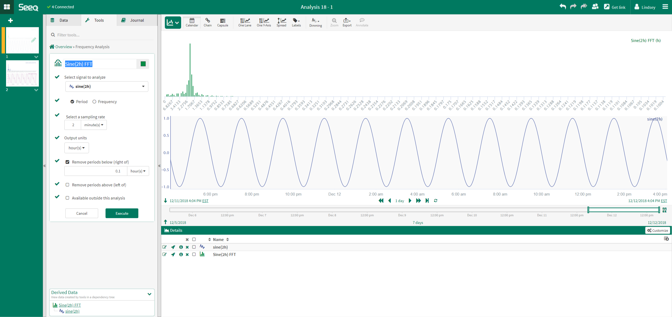
Example: Single Sine Wave
In the example to the right, the signal analyzed is a simple sine wave. When the FFT analysis is performed on this signal, the results show that there is a dominant period, or a peak, at 2 hours. This time corresponds to the period of the sine wave.
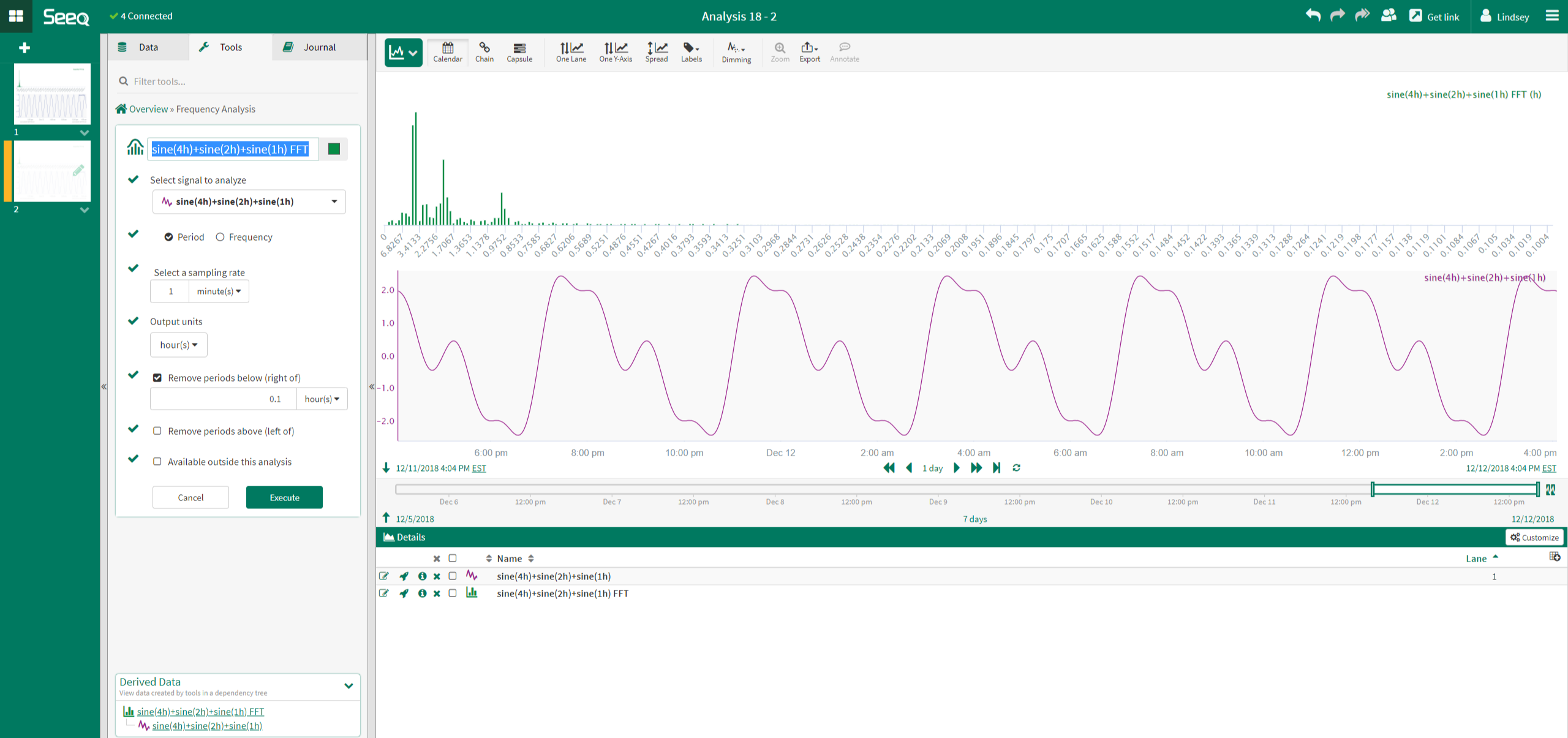
Example: Multiple Sine Waves
In the example to the right, the signal analyzed is a combination of 3 sine waves, each with a different period. When the FFT analysis is performed on this signal, the results show a dominant period, or a peak, at 1 hour, 2 hours and 4 hours. These times correspond to the periods of the 3 sine waves used to create the signal.
Note that the size of the peaks in the FFT analysis varies. The size of the peak is proportional to the amplitude of the sine wave at the corresponding period. In this example, the sine wave with the 4 hour period has the largest amplitude, then the 2 hour sine wave and finally the 1 hour sine wave.
DC Offset Considerations
Most signals have a zero-frequency component, also known as a DC offset. DC is the acronym for Direct Current in electrical systems. The DC offset is the amount that the signal is shifted above or below the axis; mathematically this is the mean amplitude of a wave signal. There is an undesirable effect of DC offset; when FFT analysis is performed on a signal with a large DC offset, the calculated FFT shows a large peak at 0, masking or "washing out" the frequencies of interest.
When performing the FFT analysis on a signal with a large DC offset, considerations must be made to remove the zero-frequency/DC offset to accurately analyze the signal and identify peak frequencies of interest.
In the example to the right, the FFT analysis is performed on a temperature signal with a large DC offset. Though the signal appears to have a dominant frequency of 1 day, the FFT analysis shows the largest, most dominant peak is at 0 and the 1 day peak is not obvious. This peak at 0 is a result of the large DC offset.
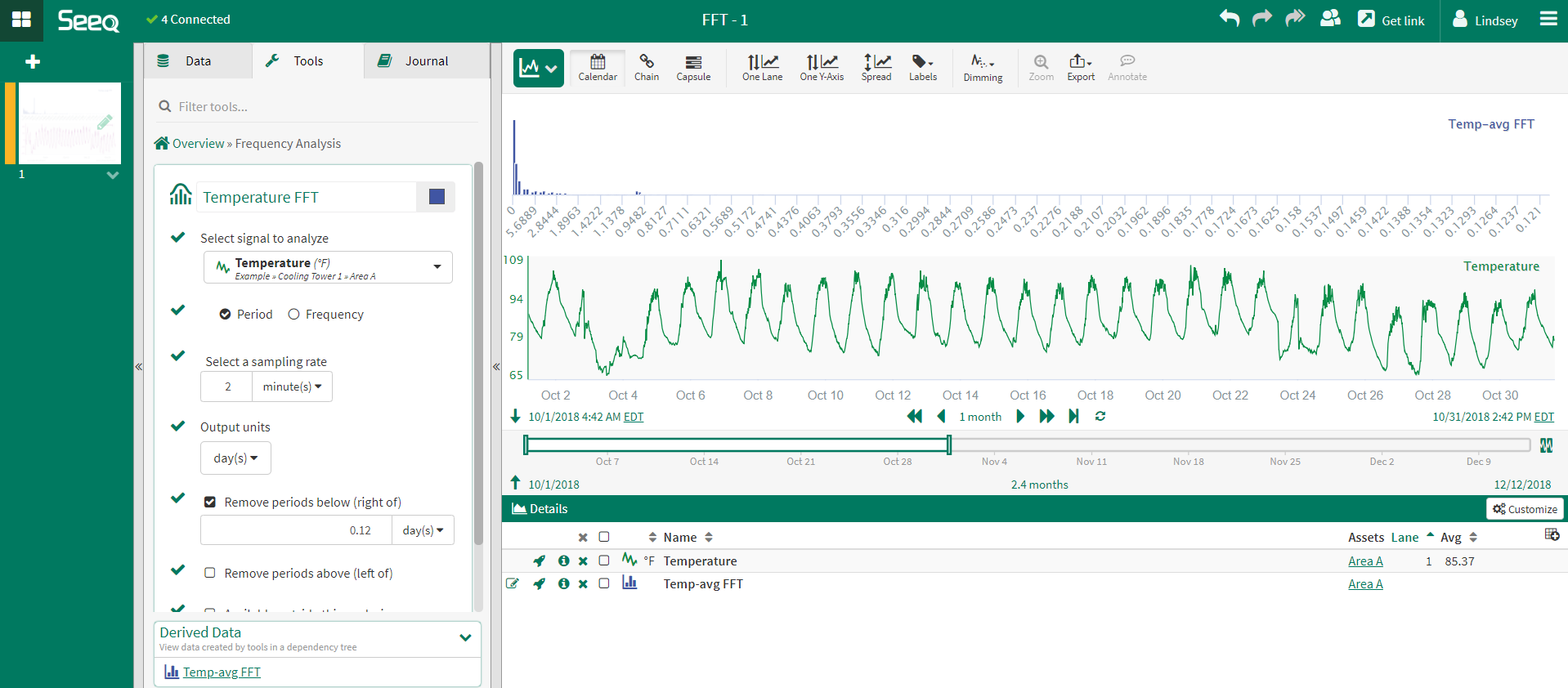
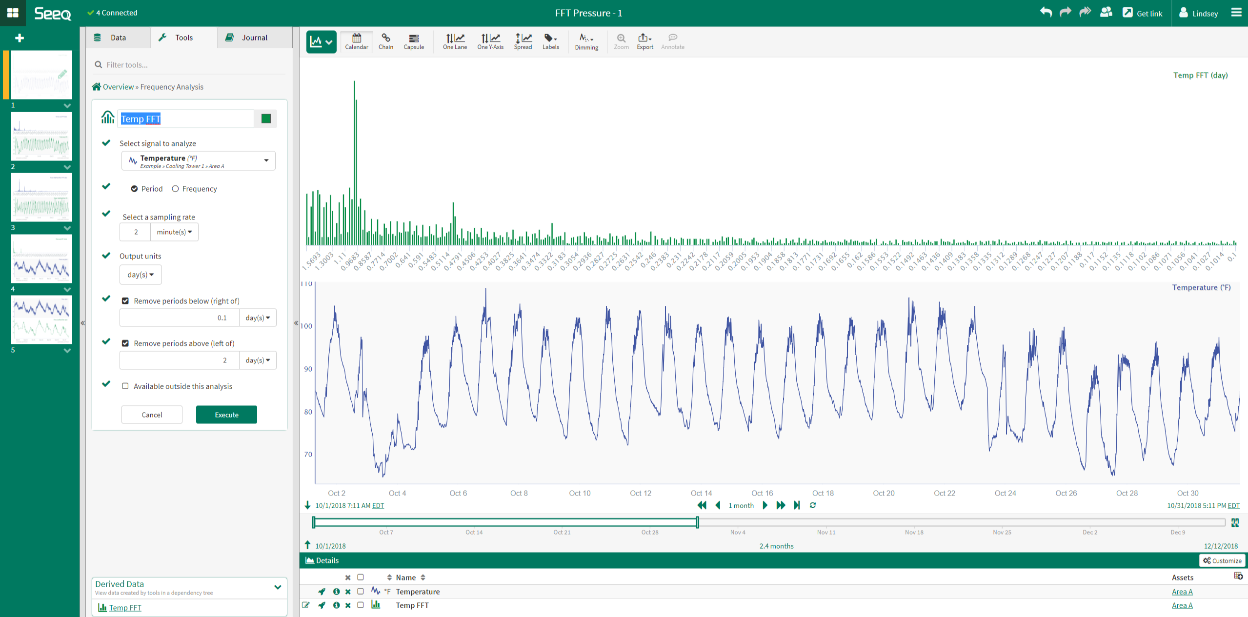
It is possible to "filter" out the effects of the DC offset by removing periods from the display; this is done from the Frequency Analysis tool menu. When these settings are adjusted, the peak period at 1 day is clear. Using this method is dependent upon the analyst knowing the range of frequencies of interest.
In many cases, adjusting these settings is sufficient to identify the dominant frequencies in the signal. However, if the dominant frequencies are still masked, the DC offset must be removed from the signal prior to performing the FFT analysis.
Remove DC Offset
There are two methods for removing the DC offset of a signal:
- Subtract the mean from the original signal
- Apply a high pass filter to the original signal
While both of these methods are described in the following subsections, using a High Pass Filter is the preferred method for removing DC offset from an input signal.
Subtract the Mean
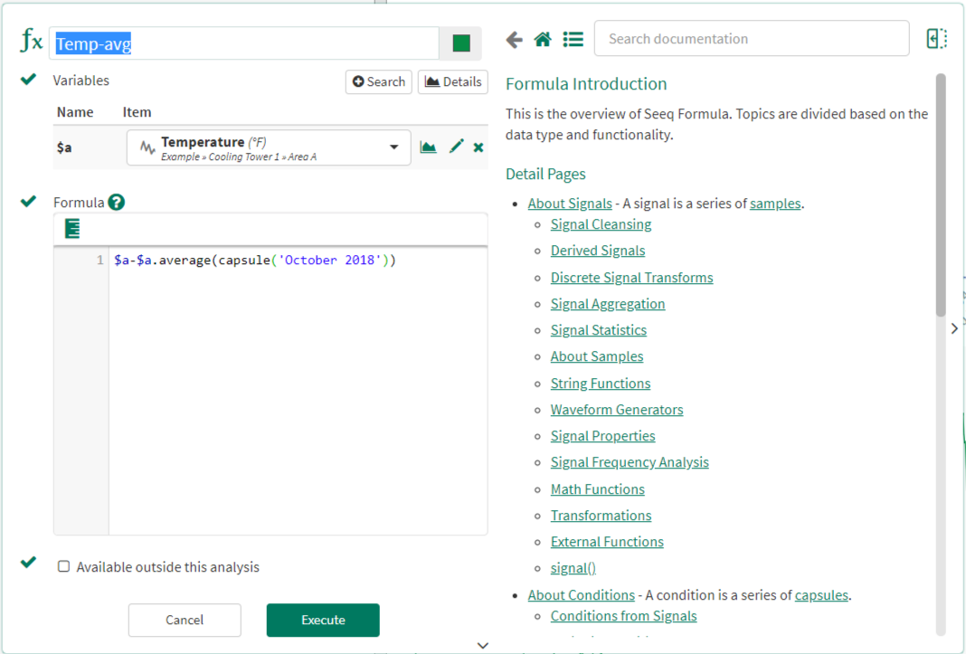
In Seeq, the mean of a signal can be subtracted from the original signal via the Formula tool. This creates a new signal, "Temp-avg" in this case, that is the original Temperature signal minus the Temperature mean for the month of October 2018.
Note: If the analyst wishes to perform the analysis over a different date range, this formula must be updated to reflect the new time range of interest. For this reason, the High Pass Filter is the preferred method.
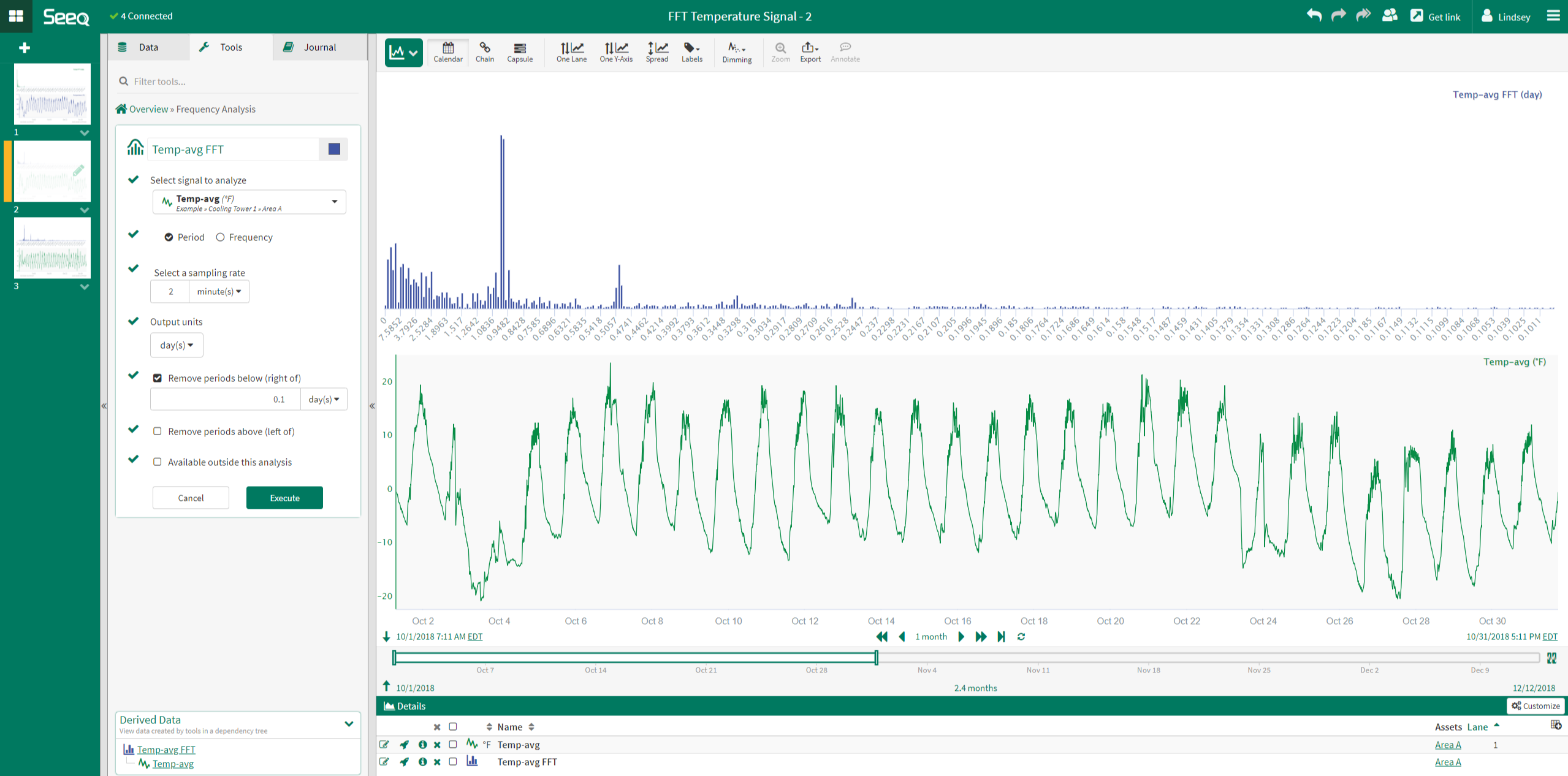
When the FFT analysis is performed on the new signal, with the DC offset removed, the result clearly shows a dominant peak at about the 1 day period.
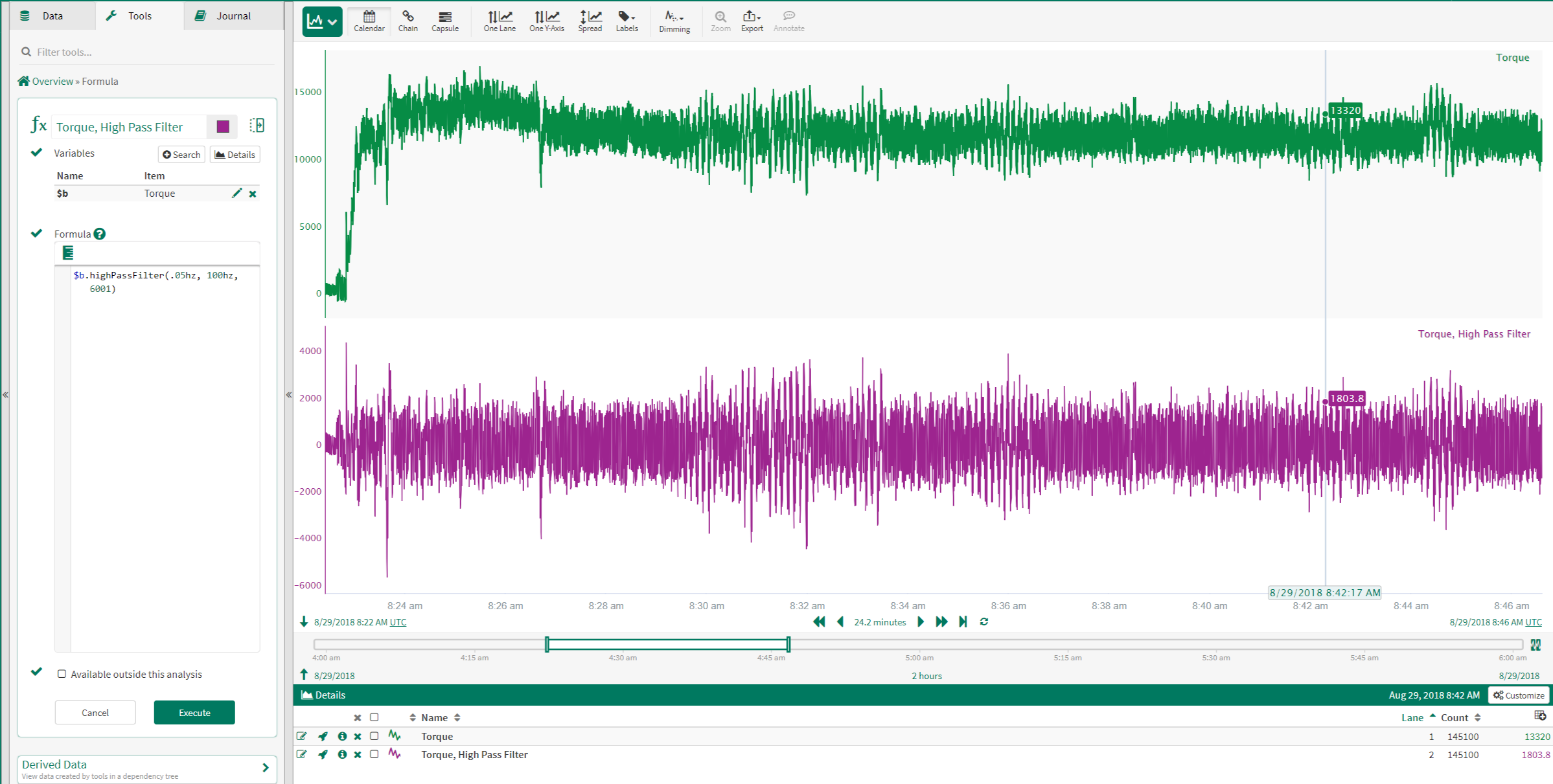
High Pass Filter
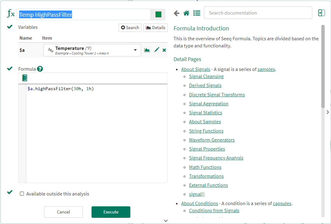
In Seeq, a High Pass Filter can be applied to a signal via the Formula tool. This creates a new signal, "Temp HighPassFilter" in this example, that is the original Temperature signal with the High Pass Filter applied.
Note: If the analyst wishes to perform the analysis over a different date range, the High Pass Filter is automatically applied to whatever date range is displayed on the trend in Seeq, and no adjustment is required to the formula. For this reason, the High Pass Filter is the preferred method for removing the DC offset from an input signal.
When the FFT analysis is performed on the new signal, with the DC offset removed, the result clearly shows a dominant peak at about the 1 day period.
.png?inst-v=58571fb4-8d41-40ca-9e05-8259c2338764)
Formula Functions
Along with Frequency Analysis in the Tools menu, there are functions in Formula that may be used to calculate different aspects of the FFT analysis, such as Peak Frequency, Power Percentage, and RMS Power. Similiar to the FFT analysis, the amount of DC offset must be considered prior to using these functions. It is best practice to either:
- Use the function on a specific band of frequencies OR
- Remove the DC offset from a signal before using these functions.
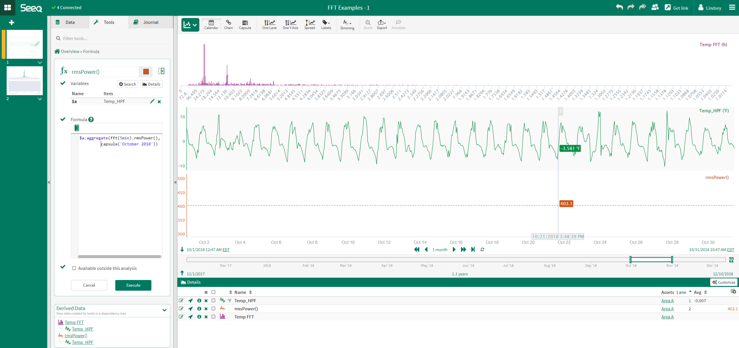
rmsPower()
This function computes the power in the user specified band of frequencies. The value is reported as the root mean square (RMS) of the frequencies in the specified band.
In the example to the right, the RMS power is calculated for a temperature signal over all frequencies. Prior to performing this function, the DC offset was removed from the temperature signal. An RMS power of ~403 is calculated.
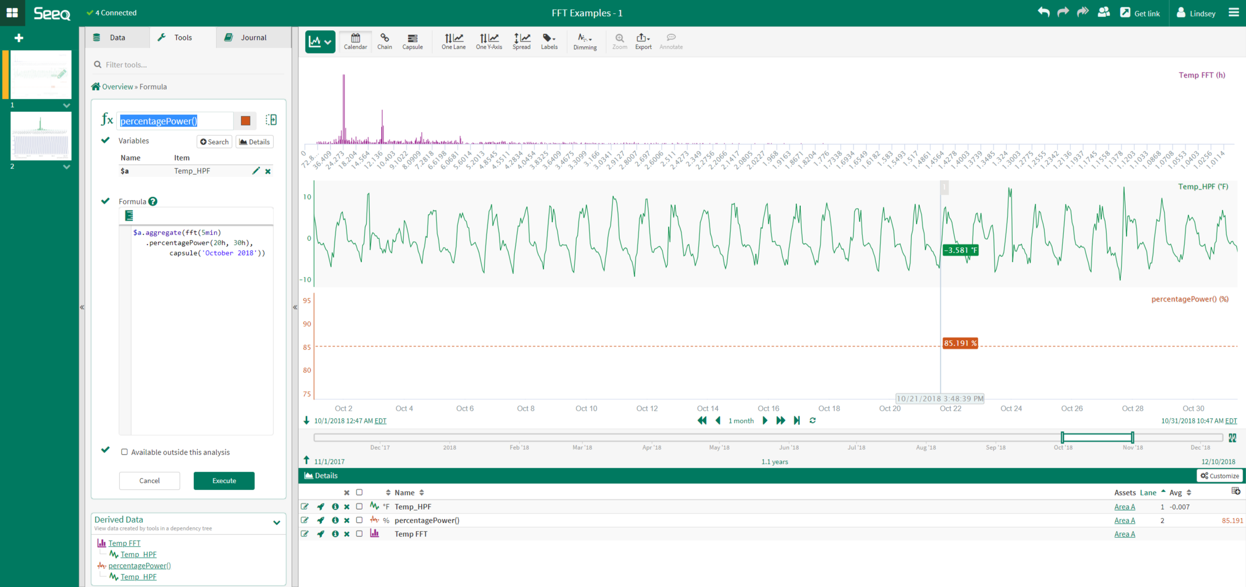
percentagePower()
This function computes the percentage power in a band of frequencies. This is the ratio of the RMS of the frequencies in the band of interest to the RMS power of the entire range.
In the example to the right, the percentage power is calculated for a temperature signal. Prior to performing this function, the DC offset was removed from the temperature signal. A percentage power of about 85% is calculated.
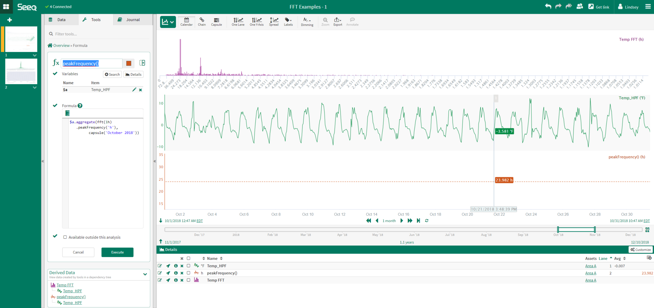
peakFrequency()
This function is used to compute the period of the peak in the FFT analysis. The result is a quadratic interpolation of adjacent bin frequencies.
In the example to the right, the peak frequency is calculated for a temperature signal. Prior to performing this function, the DC offset was removed from the temperature signal. A peak period of about 24 hours is calculated.
Time Series Data Examples
The following examples apply the Frequency Analysis tool in Seeq to common Use Cases.
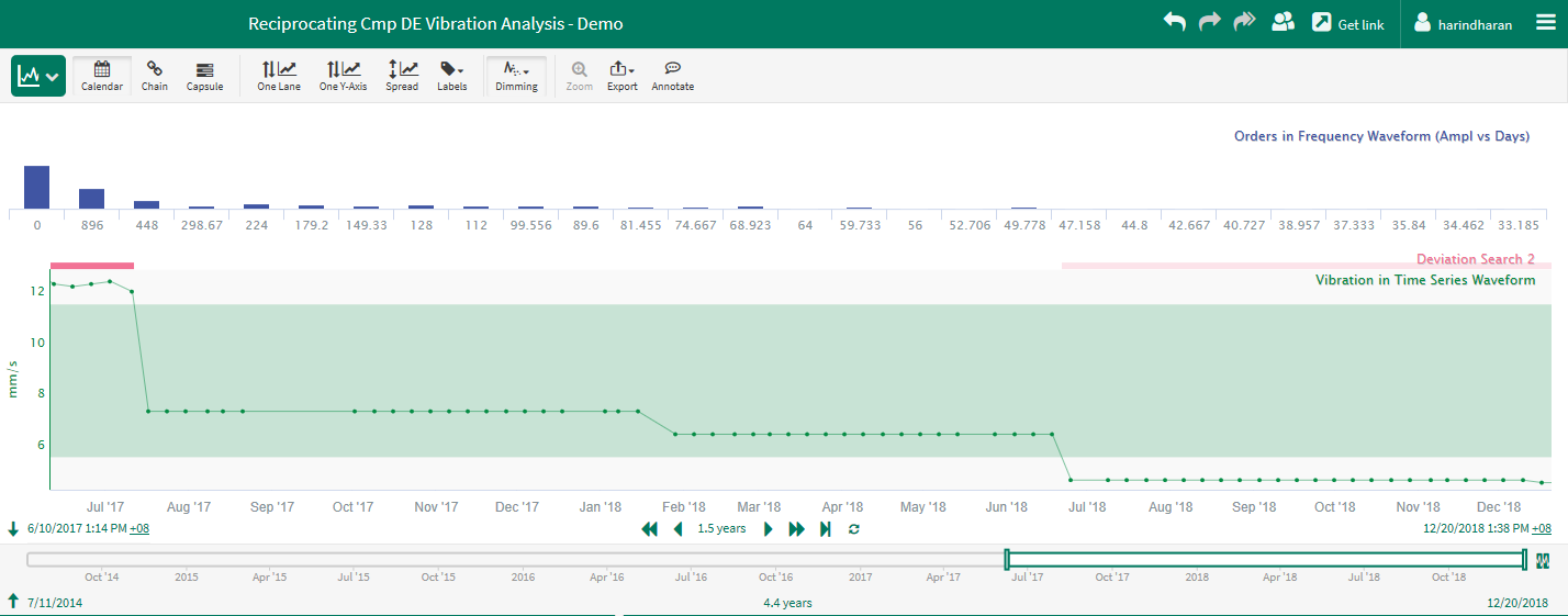
Example: Vibration Analysis
In vibration analysis, the dominant frequency of a signal is monitored over time to identify faults in rotating equipment.
Before the Frequency Analysis is performed for the signal to the left, it is first adjusted to remove the DC offset.
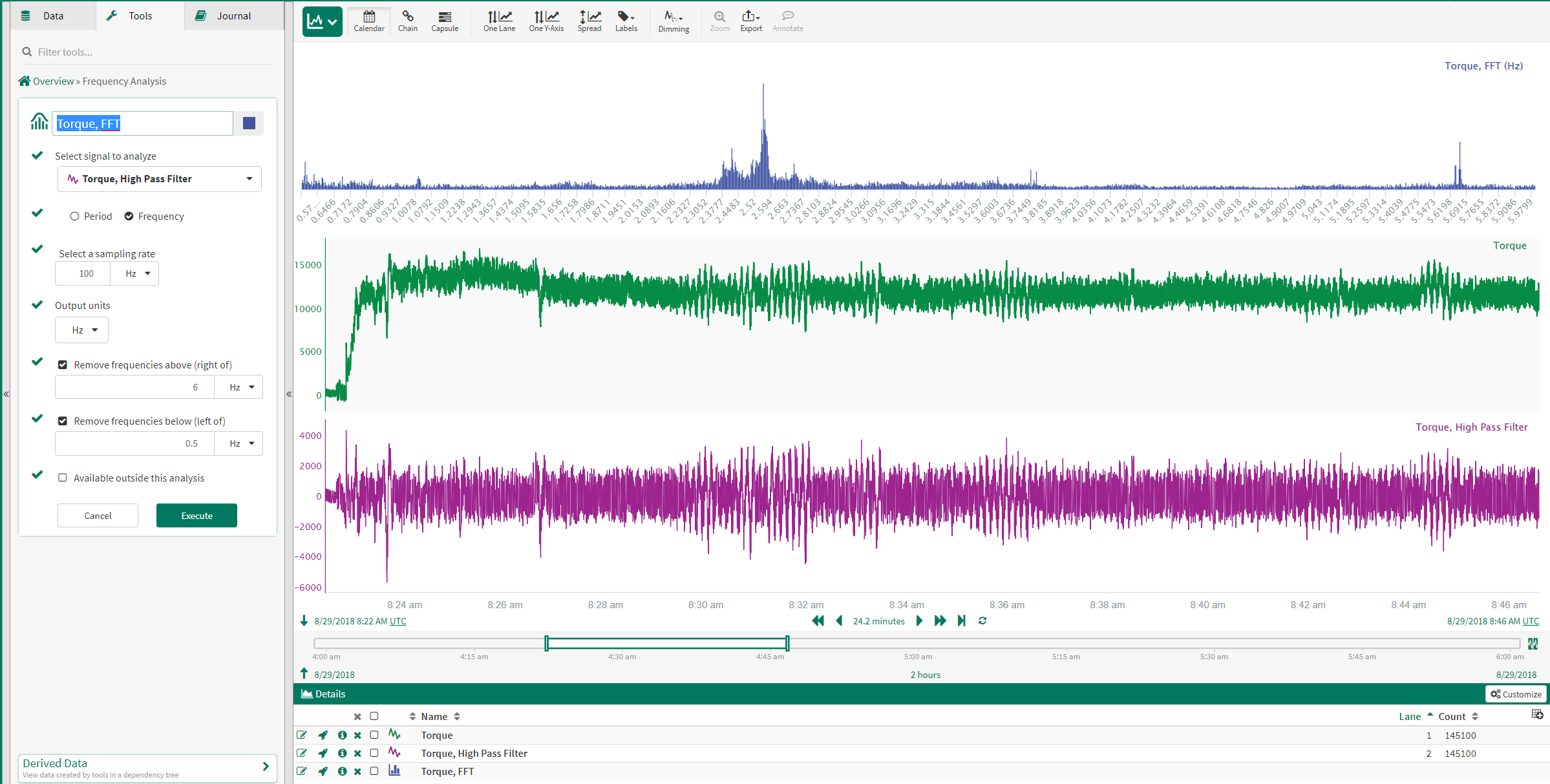
When the Frequency Analysis is performed on this signal, a peak between 2 and 3 Hz is identified.
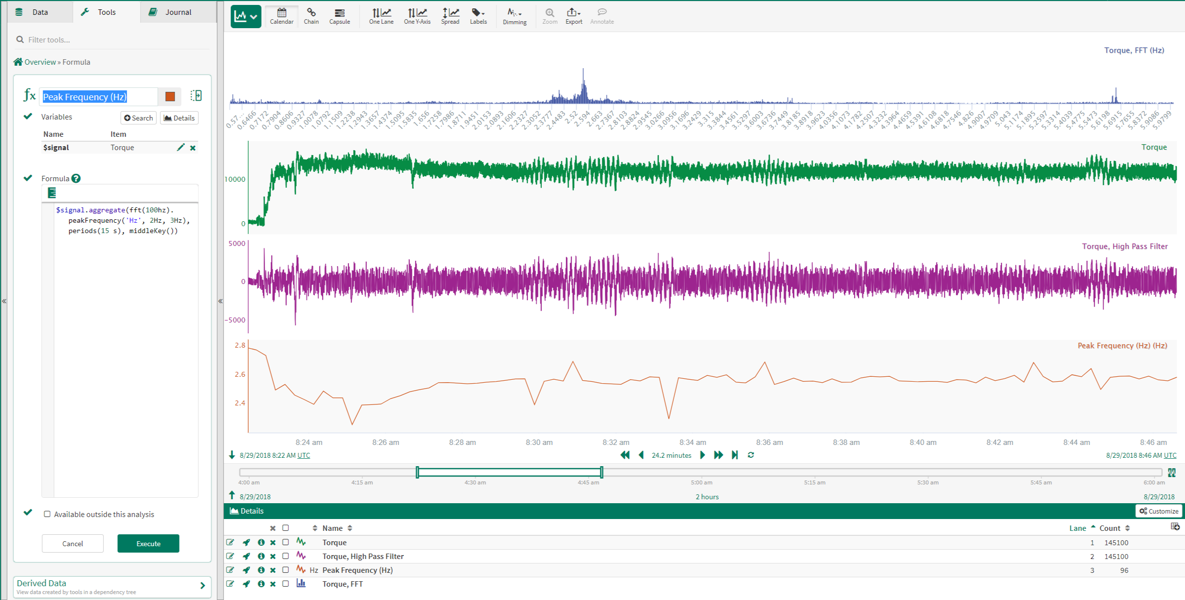
To determine if this frequency changes with time, the Peak Frequency function in Formula is used:
$signal.aggregate(fft(100hz).peakFrequency('Hz',2Hz,3Hz), period(15 s), middleKey())
This function creates a new signal that trends the peak frequency over time, calculating a new value every 15 seconds. In the trend shown to the left, once the process reaches a steady operating level, the calculated peak frequency gradually increases. This indicates that the signal is vibrating with a higher frequency.
Example: Filter Signal Noise
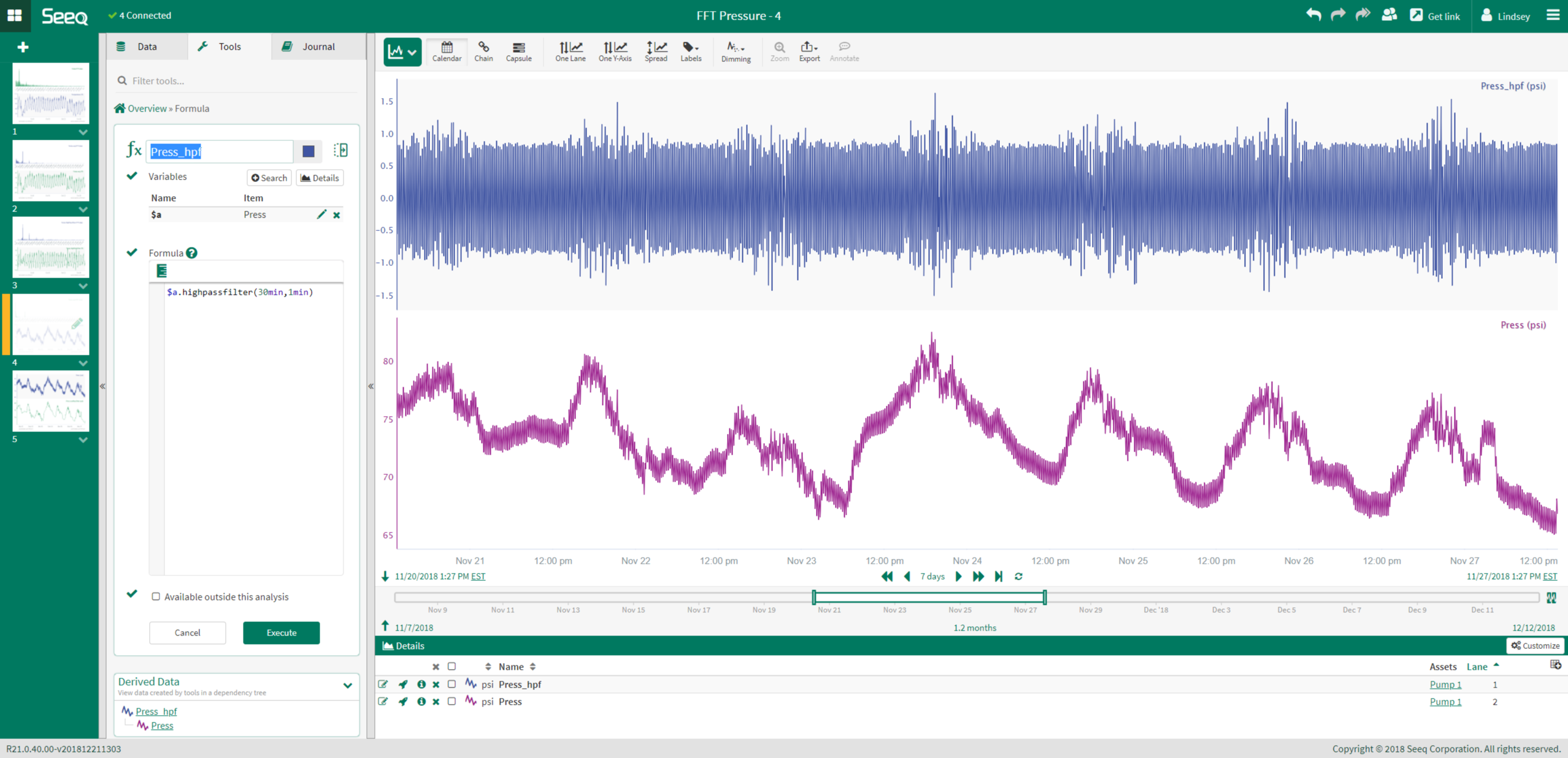
In this example, the input is a pressure signal with high frequency noise. Before applying a filter to this signal to remove the noise, FFT analysis is used to determine an appropriate cutoff for a Low Pass Filter.
The first step to performing the FFT analysis is to remove the DC offset.
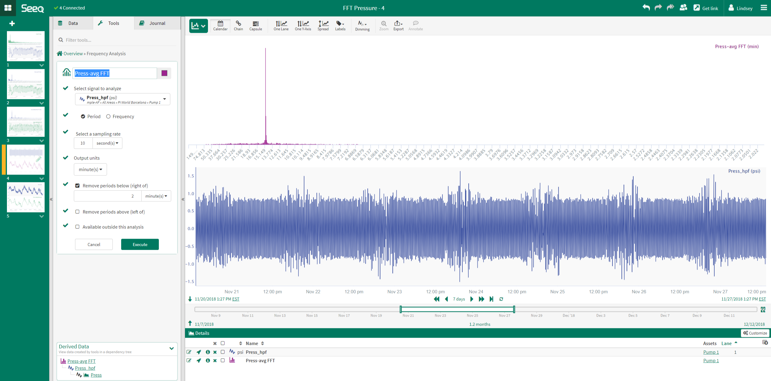
The FFT analysis reveals that there is a dominant period, or a peak, at about 15 minutes. Therefore, in order to filter this noise from the original signal, a Low Pass Filter with a cutoff period greater than 15 minutes must be used.
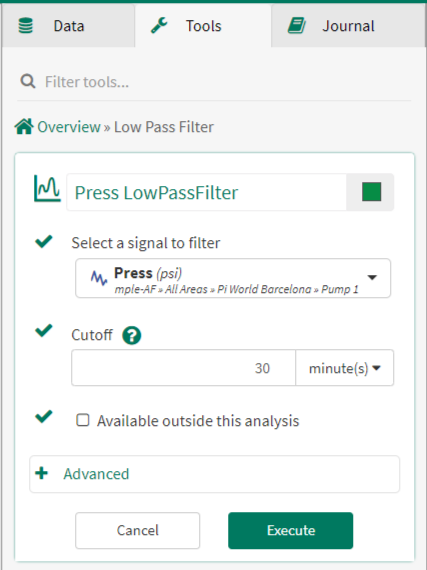
Based upon the results of the FFT analysis, a Low Pass Filter with a 30 minute cutoff is applied to the pressure signal. This filtered signal (green) shows that the high frequency noise is successfully removed.
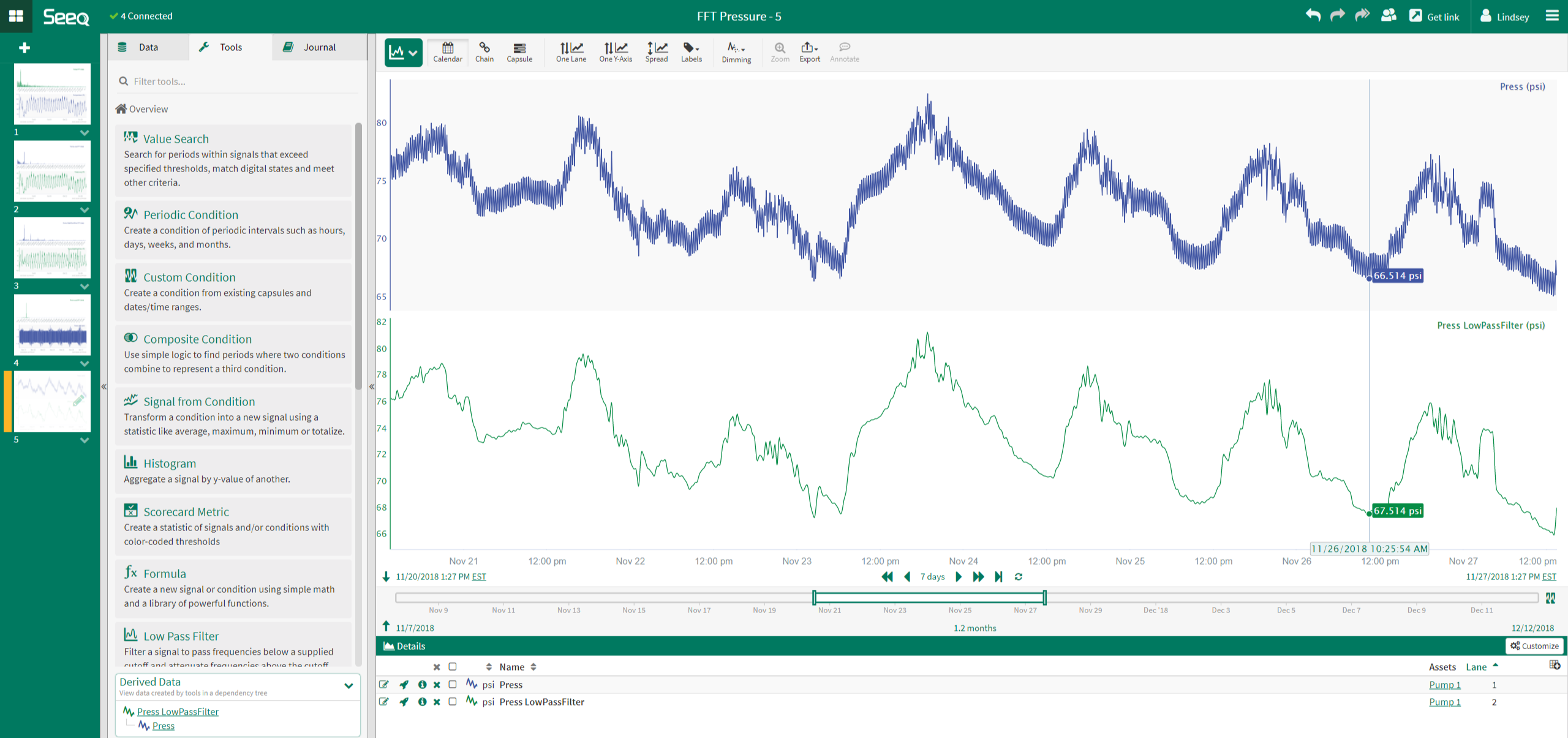
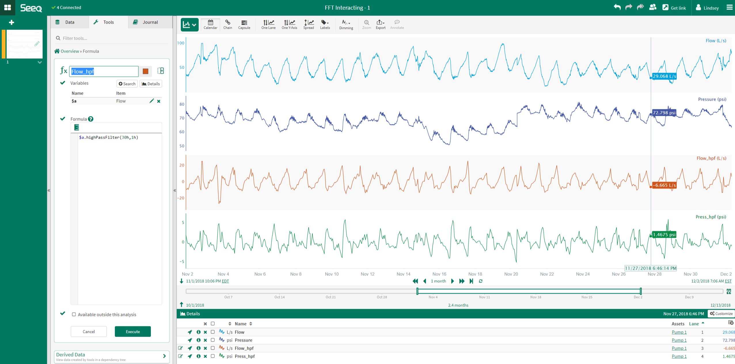
Example: Interacting Signals
In this example, there are two input signals: a flow signal and pressure signal. FFT analysis can be used to determine if these signals share a dominant peak at the same period.
The first step, before performing the FFT analysis, is to remove the DC offset.
The FFT analysis is then performed on the two signals. The results reveal that both signals have a dominant peak at a period of about 1 day.
This information highlights that the two signals may be related. This information, along with process knowledge, can be used to investigate potential process interactions or disturbances.
This type of analysis can be extended to all the signals in a unit or plant to 1) group all signals with a common disturbance and 2) help quantify the improvement to be gained by eliminating the common disturbance.
Example: Detecting Forcing & Dominant Frequencies
In this example, a time series waveform is converted to a frequency waveform using the Frequency Analysis tool in Seeq.
The image to the left shows a time series trend converted into frequency trend. This information helps a user to identify the dominant frequencies and any forcing frequencies present in the signal.