Filtering for Feature Isolation

Many analyses require finding features in a signal that cannot be isolated using a Value Search. While there are numerous ways to make features stand out, filtering is robust, fast, and easy to update once a starting point for the parameters has been determined.

This article works an example using a band pass filter to identify a low-amplitude feature that indicates a particular mode of operation in a batch process. It will demonstrate how to set up the problem, how to successfully determine filtering parameters, and will show some pitfalls associated with incorrect parameters.

Why Band Pass Filter?

Band pass filtering is a type of frequency filtering. Frequency filtering uses the fact that any signal can be represented by the sum of a bunch of sinusoids. If we selectively block some of those sinusoids, we can isolate things that happen at different “speeds” in the signal. In this case, we want to block most of the sinusoids and pass only those that make up the feature we are interested in.

Frequency filtering is similar to what is done in a stereo amplifier’s equalizer. The sound’s complex time signal is split into its frequency components and you selectively block or pass them based on their frequency. A band pass filter is equivalent to putting the bass and treble knobs to zero, and the mid-range ones to ten.

Band pass filtering is a combination of low pass and high pass filtering. Individually, a low pass filter passes low frequencies and blocks high frequencies, leaving only gradual changes. A high pass filter does the opposite, passing high frequencies and blocking low frequencies, leaving only rapid changes. The frequencies that are blocked are said to be in the filter’s “stop band” and those that are passed are in its “pass band.”

Analysis Goal

Let’s start with a brief intro to the example use case. We are searching for a “golden profile” that indicates a successful batch production run in a pharmaceutical process. These batches have a few characteristics that will help us identify them:

• At the start of a golden batch the power signal will drop to <4 kW.

• A small bump in the power signal (we call it a “dog ear”) just as the process reaches the shoulder of steady state.

• The batch process is terminated when power reaches 11 kW, even though it may climb slightly higher.

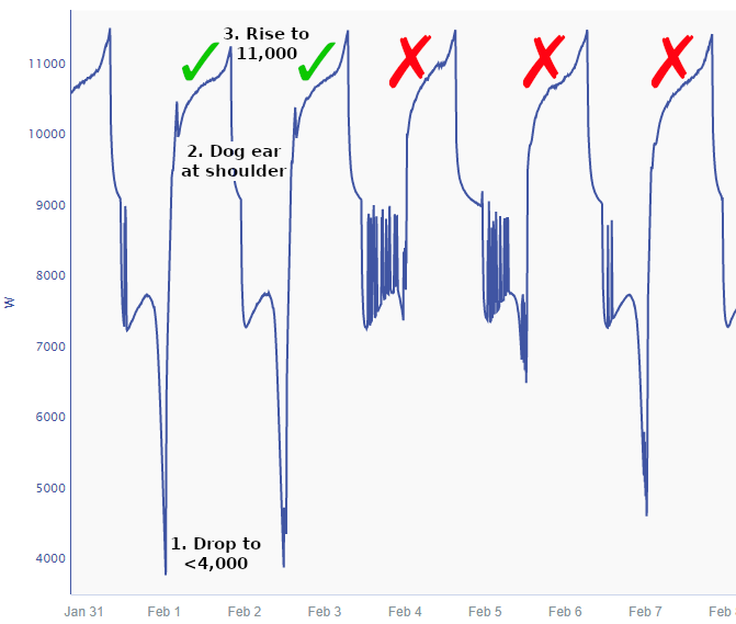
Our task is to create capsules that run from the peak of the dog ear to where the power reaches 11 kW in batches that meet the stated criteria.

Preparing Our Data for Filtering

Before filtering, we want to remove data that is not needed. The cleaner the start signal, the better. How this is done is use-case specific. Are you removing down times of a pump? Startup oscillations of a flow unit? Or, as is the case in our current example, isolating batches that could contain our golden profile?

To isolate batches that start with a drop to 4 kW, we are going to use the fact that the signal must drop below 4 kW before rising to 11 kW. This can be done using the Value Search pane, but we’ll do it in Formula because we want to modify the resulting capsules and so we can name the outputs.

Remember that spaces, new lines, and text after “//” are ignored in Formula.

$raw_power_signal.validValues()
.valueSearch(
   1d,                                // capsules are a maximum of one day in length
   isLessThan(4000), 0, true,         // start when less than 4000, for 0 minutes, start immediately
   isGreaterThan(11000), 0, true)     // end when greater than 11000, for 0 minutes, end immediately

Because the power signal can oscillate at the lowest power level, it’s advantageous to trim off the first couple of hours of the signal by shrinking the capsules and shifting them so that their ends line up again. We can do this by modifying the above Formula to include a shrink and move.

// **Formula 1** //
$trim = 2h                            // we'll trim a total of 2 hours off the capsule 
$potential_batches = $raw_power_signal.validValues()
.valueSearch(
   1d,
   isLessThan(4000), 0, true,
   isGreaterThan(11000), 0, true)
.shrink($trim/2)                      // shrink the capsules by 2h/2 from each end
.move($trim/2)                        // shift by 2h/2 to line up the trailing end again
return $potential_batches

In this articles, signals are named and returned via the return keyword to clearly indicate which signals are being referred to to later in the article. return is not for formulas, but won’t raise errors when used.

From this, we end up with capsules that contain potential batches.

We can now use Formula to retain only the data in a “potential batch” for further analysis:

$potential_batches_power_signal = $raw_power_signal.within($potential_batches)

return $potential_batches_power_signal

Low Pass Filtering

Digital filtering is a “linear process”, which means that you can apply the low and high pass filters in any order. We start with the low pass, but you could start with the high pass filter.

The first task is to identify the filter’s cutoff frequency. We’ll be working in period rather than frequency units (that is, seconds/minutes/hours rather than Hertz) since periods are easy to read from the graphs.

Seeq allows either frequency or period units. These are interchangeable as the frequency relates to period based on frequency = 1/(period in seconds). Keep in mind that the filter behaves inversely when period rather than frequency is supplied: a low pass filter passes high-period signal components, and vice versa.

If we zoom in on one of the capsules that contains a candidate batch, we see that there is some global jitter as well as a feature that is similar to our target feature. We need to remove this feature using the low pass filter. The jitter appears to be shorter period than the feature we’re removing, so will get removed by the same filter.

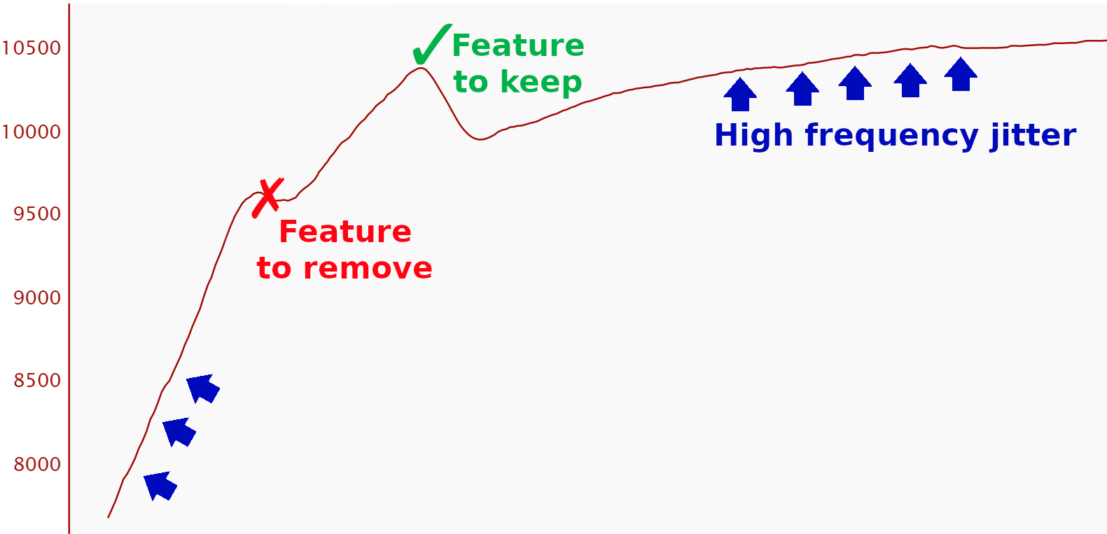
We need to be careful removing the feature with the red “X” above. It’s close enough in duration to our target feature that we might not be able to completely remove it without attenuating our target feature. This means that we’ll need to design our low pass filter carefully .

The low and high pass filters take three parameters: cutoff, period, and taps. Their use and how to select them will be explained in the following paragraphs.

To identify an appropriate cutoff, try to estimate how long a sinusiod of the same frequency as the feature you are trying to remove would take to complete one full cycle.

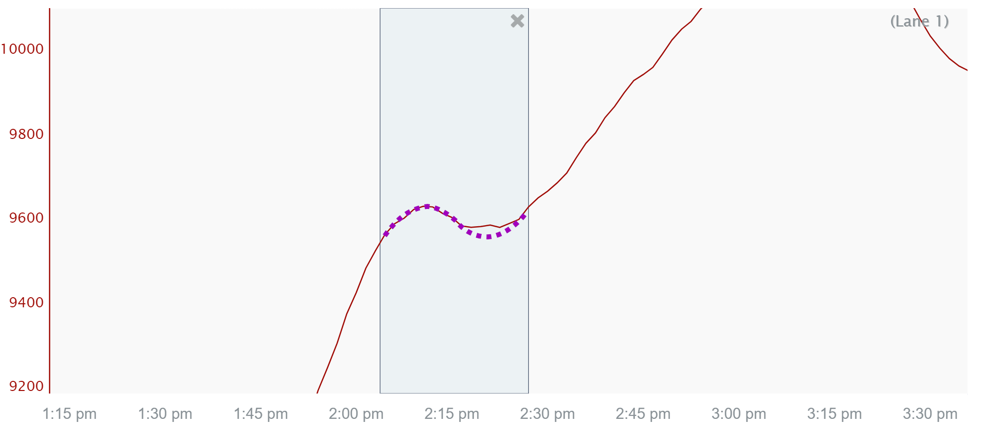
It appears to go from about 2:10pm to 2:30pm, so we’ll call it 20 minutes.

Filters have a property called roll-off which quantifies how well they attenuate frequencies near the specified cutoff. If we put our cutoff at exactly 20 minutes, we wouldn’t actually remove the feature since roll-off isn’t immediate: it’s somewhat blurred and removes some stuff that takes longer than 20 minutes and allows some stuff that takes shorter than 20 minutes. The roll-off can be optimized, but we are just going to play around with the parameters with 20 minutes as a start until we find something we like.

The blurriness of the roll-off is impacted by the amount of data used for the filter. This is controlled in Seeq using the period and taps parameters: period selects the the sampling period of the input signal and taps are the number of input samples to use. Increasing taps gives you a sharper roll-off, meaning you can be more selective about features you keep or eliminate, but makes the filter work worse at the edges of your data. Critical to know in Seeq is that if you decrease period, you must increase taps to maintain the same filter roll-off sharpness.

For more detailed information on the impact of period and taps, refer to Steven Smith’s book on digital signal processing. It’s freely available by chapters on his website. The relevant chapter for this topic can be found here.

As a starting point for our filter, we’re going to use cutoff = 10 min (half our target’s period), period = 90 seconds (same as our input signal), and taps = 33 (the default).

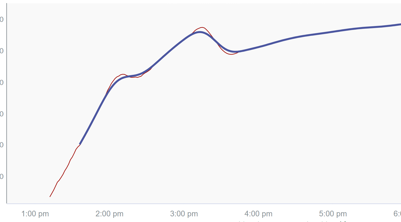
Not too bad for a first try! After playing around for a bit, we settle on increasing our taps to remove frequencies near our target frequency more precisely, and consequently be able to bring the cutoff frequency down to 45 minutes.

$low_pass_power_signal = $potential_batches_power_signal.lowPassFilter(45min, 90s, 45)

return $low_pass_power_signal

While we used a digital filter for the low pass filtering, there are other options available in Seeq, such as the sgFilter and agileFilter which have their own advantages and disadvantages. One nice thing about these filters is that they can operate as effective smoothing filters in the vicinity of data gaps; however, you lose the ability to specify the frequency that you want to retain. This is because they are technically non-linear algorithmic filters that use statistics to calculate a filtered sample value, rather than the frequency content of the signal. That said, if the performance of the lowPassFilter does not meet your needs (such as needing more data in the vicinity of data gaps), you can try using one of the others filters for the low pass filtering stage. You can find more information on the other smoothing filters in the Intro to Signal Smoothing Filters article.

High Pass Filtering

For the high pass filter, we are going to do something similar. In this case though, we are going to identify the feature we want to keep and change our filtering parameters to retain it.

Using the same process, we estimated the period of our feature at about 1 hour, so we’re going to start with twice that as the cutoff, keep period the same as the input signal, and start with taps = 33. taps and period have exactly the same relationship in high pass as they do in low pass: the higher the taps, the more surgical you can be with your filter.

Again, not a bad start. In fact, we'll keep it!

$filtered_power_signal = $low_pass_power_signal.highPassFilter(2h, 90s, 33)

return $filtered_power_signal

Note that the resultant signal has been moved to y=0. A very low frequency in the signal is its DC-offset, which is analogous to the signal’s average value. After high pass filtering, the average value of the signal will be zero, which you can see here.

Band Pass Filter by Low and High Pass Combination

Combining these two filtering operations into a single formula is as easy as chaining them together. For code readability, we’ve created parameters for the variables.

// **Formula 2** //
// low pass filter specs
$low_pass_cutoff = 45min
$low_pass_sample_period = 90s
$low_pass_taps = 45

// high pass filter specs
$high_pass_cutoff = 2h
$high_pass_sample_period = 90s
$high_pass_taps = 33

// do the filtering
$filtered_power_signal = $potential_batches_power_signal
.lowPassFilter($low_pass_cutoff, $low_pass_sample_period, $low_pass_taps )
.highPassFilter($high_pass_cutoff, $high_pass_sample_period, $high_pass_taps)

Potential Pitfalls of Chaining Filters

A couple of things to note about combining and using these filters:

• The filter cutoff period for the high pass filter needs to be higher than the cutoff period for the low pass filter. (Conversely, the cutoff frequency for the high pass needs to be lower than the cutoff frequency for the low pass.) Otherwise all you’re doing is high pass filtering data that leaked through the stop band of the low pass filter - and the results would be garbage.

• The sampling period of Seeq’s filters can be set independently. This can cause issues for high pass filtering after low pass filtering because the linear interpolation can lead to artificial high frequency content around the samples due to the rapid change of slope. For this reason, the high pass sampling period should be greater than or equal to the input signal sampling period.

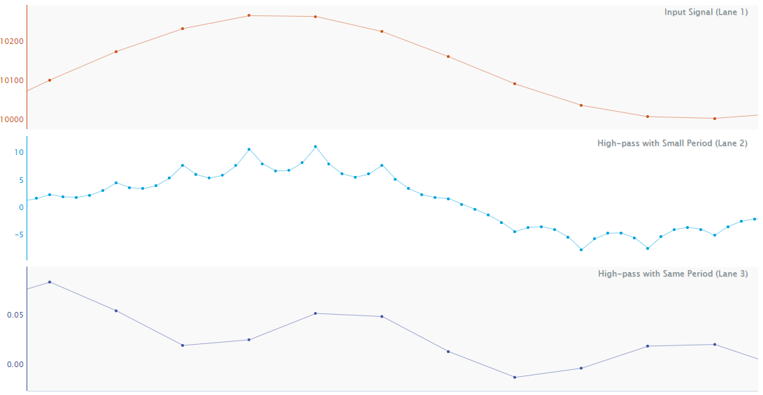
As an example, in this image you can see two major effects of the sampling period selection. The signals are

• Top: The input signal with a sampling period of 5 minutes;

• Middle: A high pass filter with cutoff = 20 min, period = 1 min, and taps = 33;

• Bottom: A high pass filter with cutoff = 20 min, period = 5 min, and taps = 33.

The first thing to notice is the attenuation of the low frequency component (the long wave), which has an amplitude of about 100 in the top, 15 in the middle, and is essentially removed in the bottom signal. This is because the low period in the middle signal leads to that blurry filter roll-off, letting a significant portion of the low frequency stuff through. The higher period with the same number of taps in the bottom signal sharpens the roll-off, leading to almost no low frequency content.

The second thing to notice is the interpolation issue. With a one-minute period you can see the “peaks” created at each input sample in the middle signal. These are clearly wrong and can be avoided by not over sampling when high pass filtering.

Creating a Condition from the Band Pass Features

Now that we have completed the filtering, we will complete our task of creating capsules that start at the dog ears and ending at the 11 kW level. The process will be:

1. Find the peaks in $filtered_power_signal .

2. Eliminate $potential_batches capsules that don’t contain a high enough peak.

3. Create capsules within the remaining data that start at the peak and end at 11 kW.

Finding Peaks in the Filtered Power Signal

Up to now, we’ve used filtering to create a signal that has high amplitude at the time of the dog ears and low amplitude elsewhere. Now we want to use this signal to create capsules that start at the dog ears and end when the signal reaches 11kW.

There are variety of dog ears sizes, which correspond to different amplitude peaks in the filtered signal. We can select different size dog ears by changing the size of the peak we select in the filtered signal. This way we have flexibility in what constitutes a sufficiently large “dog ear”. We played around and settled on a cutoff value in the filtered signal of 25. Using that, we then created a new signal with samples at the peaks of the dog ears.

// **Formula 3** //
$dog_ear_cutoff = 25
$dog_ear_peaks = $filtered_power_signal
.aggregate(                                                     // create a new signal
    maxValue(),                                                 // with values of the max value
    $filtered_power_signal.valueSearch(1d, 
      isGreaterThan($dog_ear_cutoff)),                          // in these capsules
    maxKey())                                                   // with a timestamp of the max value

return $dog_ear_peaks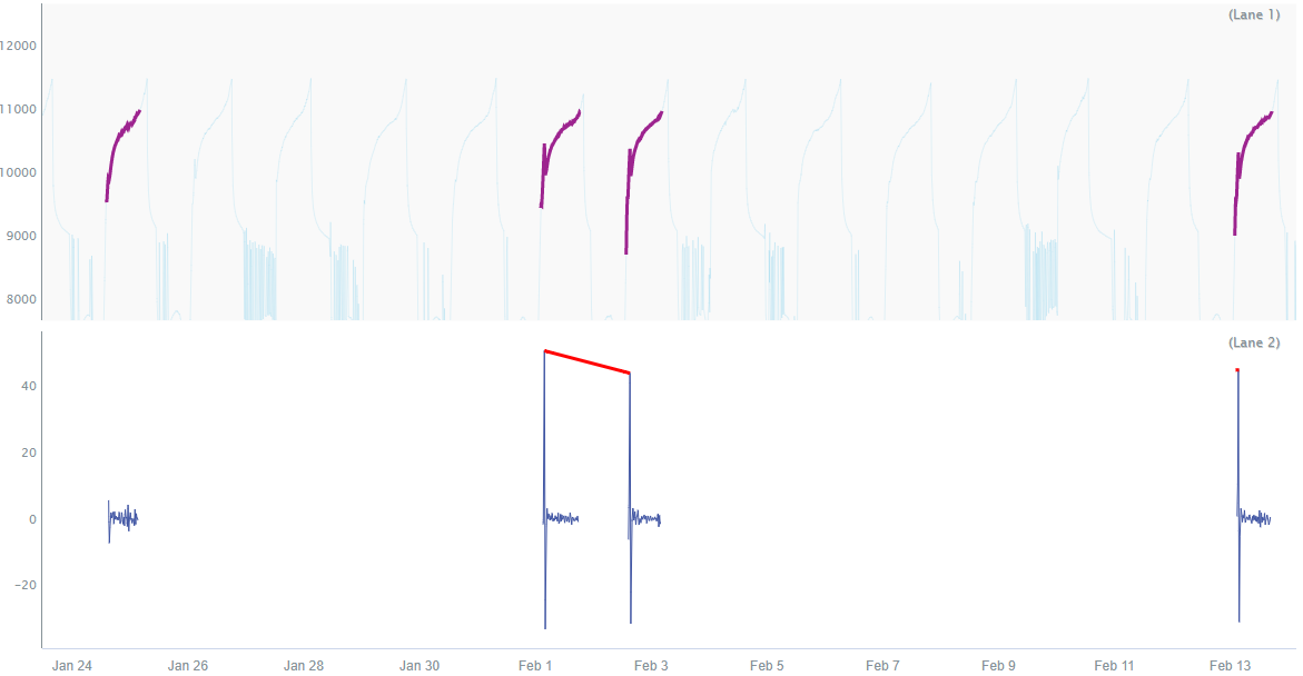

Eliminating Potential Batches without a Dog Ear

To eliminate the batches that do not have a large enough peak to count as a dog ear, new capsules are created that start 4 hours before the peak of the dog ear and end at the peak. Then only the potential batches that intersect with these new capsules were selected.

$capsule_duration = 4h                        // the duration of the dog ear capsules

$dog_ear_capsules = $dog_ear_peaks
.transformToCapsules(                         // convert the samples to capsules
    $sample -> capsule(                       // each capsule will be have a: 
        $sample.getKey()-$capsule_duration,   // start time of the sample time - the duration 
        $sample.getKey()),                    // and an end time of the duration
        $capsule_duration)                    // with a maximum duration of the duration
        
return $dog_ear_capsules

// eliminate potential batches that are not overlapped by a dog ear capsule
$dog_ear_batches = $potential_batches.overlappedBy($dog_ear_capsules)

return $dog_ear_batches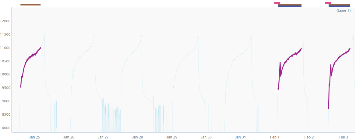

In this view, you can see that the two batches on the right remain (the blue capsules), since they overlap the dog ear capsules (the pink capsules), while the one on the left was eliminated (no pink or blue capsules).

Trimming the Dog Ear Batches to Start at the Dog Ear

We then trimmed the potential batches using the dog ear capsules so that the batch capsules start at the peak of the dog ear. This left us with only the golden batches, which was our original goal.

$golden_batches = $dog_ear_batches.minus($dog_ear_capsules)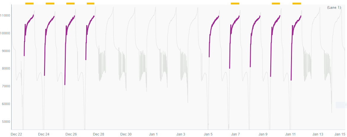

Reporting

To report our batches, we are gong to create a Scorecard Metric that counts the number of batches in a given week and puts them in a table with headings of “<year> Week <week number>” (e.g., “2018 Week 16”). The metric item will be the golden batches condition, with a statistic of Count, and a weekly periodic condition.

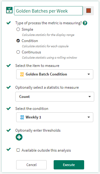
In the created table, we’re going to edit the Headers to show the start time only, with a Date Format of YYYY [Week] WW to get the format we want.

And there you have it!

Summary

In this document we used band pass filtering to isolate a feature, then used that feature to create capsules that contained our golden batches. Finally we reported our weekly golden batch rates using a Scorecard Metric.

Band pass filtering is a useful tool for narrow frequency-band feature isolation, especially if you know or can estimate the frequency of the feature you’re looking for.

Benefits of the band pass method:

• Few intermediate signals required.

• Flexible selection of the dog ears by changing the cutoff in Formula 3.

Things to watch out for:

• Selection of the filter parameters cutoff, period, and taps are all important to the final result. When filtering data, you should spend time playing with the parameters and observing their impact.

• A greater period and higher number of taps improves filter performance, but this must be balanced with the need for filtering close to gaps.

Once you get a feel for how to start your selection and recognize when you’re moving in a good direction, creating filters becomes easy…and kinda fun! 😉